Perceptron: Learning Linear Classification Through Machine Monitoring

Learning Objectives

By the end of this lesson, you should be able to:

1. Explain what a Perceptron does.
2. Understand why it uses $w^Tx+b$.
3. Explain why the update rule is $w \leftarrow w+\eta yx$.
4. Perform a Perceptron update by hand.
5. Identify the main limitations of a Perceptron.
6. Match each limitation with a later improvement.
7. Train a Perceptron with scikit-learn.

---

1. Problem: Should a Machine Trigger an Alarm?

Suppose a factory monitors a machine using two sensors:

• $x_1$: temperature deviation from the normal level
• $x_2$: vibration deviation from the normal level

A machine state is represented by:

$$x= \begin{bmatrix} x_1\\ x_2 \end{bmatrix}$$

For example:

$$x= \begin{bmatrix} 2\\ 1 \end{bmatrix}$$

means that both temperature and vibration are above their normal levels.

The label is:

$$y= \begin{cases} +1 & \text{trigger an alarm}\\ -1 & \text{do not trigger an alarm} \end{cases}$$

Example training data:

This is a binary classification problem because there are only two possible outputs.

The goal is to learn a rule from known examples and use it to classify a new machine state.

---

2. The Basic Idea

A Perceptron first calculates a score:

$$s=w^Tx+b$$

where:

• $x$ is the feature vector
• $w$ is the weight vector
• $b$ is the bias
• $s$ is the decision score

For two features:

$$s=w_1x_1+w_2x_2+b$$

The score is converted into a prediction:

$$\hat y= \begin{cases} +1 & s>0\\ -1 & s\leq0 \end{cases}$$

Equivalently:

$$\hat y=\operatorname{sign}(w^Tx+b)$$

The model therefore performs two steps:

1. Combine the features into one score.
2. Use the sign of that score to choose a class.

---

3. Why Use a Weighted Sum?

The expression:

$$w^Tx$$

is a dot product:

$$w^Tx=w_1x_1+w_2x_2+\cdots+w_dx_d$$

Each weight describes how one feature affects the final score.

Suppose:

$$w= \begin{bmatrix} 1.5\\ 0.5 \end{bmatrix}$$

Then:

$$s=1.5x_1+0.5x_2+b$$

This means:

• increasing temperature deviation by one unit increases the score by 1.5
• increasing vibration deviation by one unit increases the score by 0.5

A negative weight would mean that increasing the feature lowers the score.

Therefore, each weight represents:

1. The direction of the feature's effect.
2. The strength of the feature's effect.

---

4. Why Do We Need the Bias?

Without a bias, the model would use:

$$s=w^Tx$$

The decision boundary would always pass through the origin.

That is too restrictive for many problems.

For example:

$$x_1+x_2>3$$

can be rewritten as:

$$x_1+x_2-3>0$$

Therefore:

$$w= \begin{bmatrix} 1\\ 1 \end{bmatrix}, \qquad b=-3$$

The weights control the direction of the decision boundary.

The bias controls where the boundary is placed.

---

5. The Decision Boundary

The decision boundary is the set of points where:

$$w^Tx+b=0$$

With two features, it is a line.

The line separates the plane into two regions:

$$w^Tx+b>0$$

is predicted as $+1$, while:

$$w^Tx+b<0$$

is predicted as $-1$.

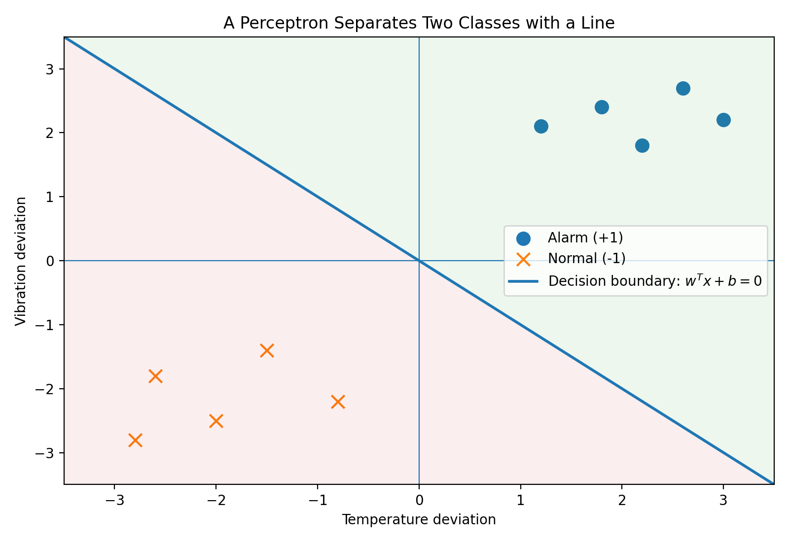A linear Perceptron decision boundary

The weight vector $w$ is perpendicular to the decision boundary.

Therefore:

• changing $w$ changes the direction of the boundary
• changing $b$ shifts the boundary

---

6. A Prediction Example

Suppose:

$$w= \begin{bmatrix} 1\\ 1 \end{bmatrix}, \qquad b=0$$

A new machine has:

$$x= \begin{bmatrix} 1.2\\ 0.7 \end{bmatrix}$$

The score is:

$$s=w^Tx+b$$ $$=1.2+0.7$$ $$=1.9$$

Since:

$$1.9>0$$

the prediction is:

$$\hat y=+1$$

The machine should trigger an alarm.

---

7. How Does the Perceptron Learn?

At the beginning, the model does not know the correct $w$ and $b$.

A common initialization is:

$$w=0, \qquad b=0$$

For each training example $(x_i,y_i)$, the model calculates:

$$s_i=w^Tx_i+b$$

If the prediction is correct, it does nothing.

If the prediction is wrong, it updates:

$$w\leftarrow w+\eta y_ix_i$$ $$b\leftarrow b+\eta y_i$$

where $\eta>0$ is the learning rate.

---

8. How Do We Detect a Mistake?

A mistake is detected using:

$$y_i(w^Tx_i+b)\leq0$$

Why does this work?

If $y_i=+1$, the score should be positive.

If $y_i=-1$, the score should be negative.

In both cases, a correct prediction satisfies:

$$y_i(w^Tx_i+b)>0$$

Therefore:

$$y_i(w^Tx_i+b)\leq0$$

means that the example is misclassified or exactly on the boundary.

The value:

$$y_i(w^Tx_i+b)$$

is called the signed margin.

It tells us whether the example is on the correct side of the boundary.

---

9. Why Is the Update $w+\eta yx$?

The update rule is designed to improve the classification of the current misclassified example.

9.1 Misclassified Positive Example

Suppose:

$$y_i=+1$$

Then:

$$w_{\text{new}}=w+\eta x_i$$

For the same example:

$$w_{\text{new}}^Tx_i = (w+\eta x_i)^Tx_i$$ $$= w^Tx_i+\eta x_i^Tx_i$$

Since:

$$x_i^Tx_i=\lVert x_i\rVert^2\geq0$$

the score increases.

The model becomes more likely to classify that example as positive next time.

9.2 Misclassified Negative Example

Suppose:

$$y_i=-1$$

Then:

$$w_{\text{new}}=w-\eta x_i$$

The score for that example decreases.

The model becomes more likely to classify it as negative next time.

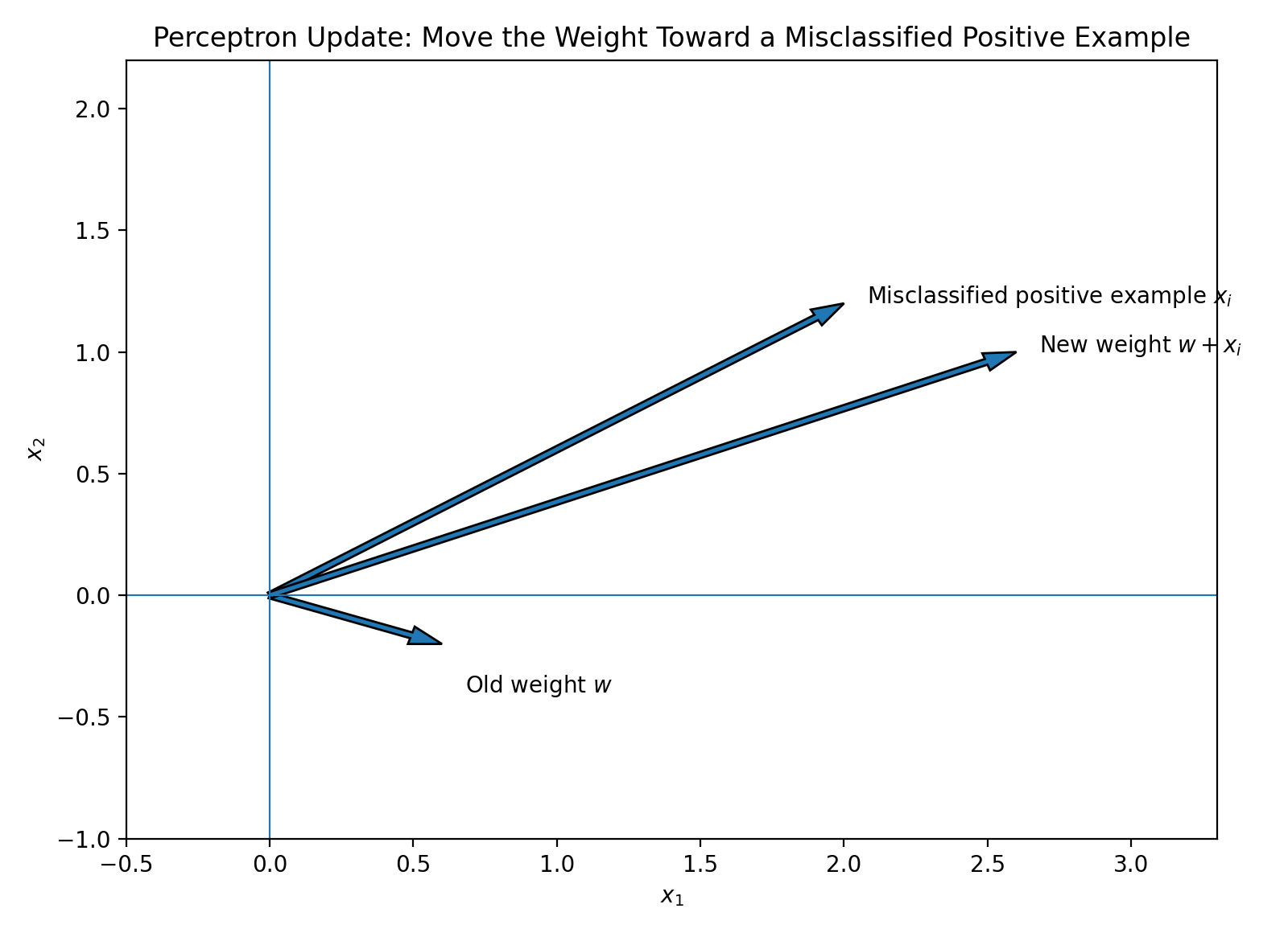Perceptron weight update intuition

---

10. Mathematical Reason for the Update

Before the update:

$$m_{\text{old}}=y_i(w^Tx_i+b)$$

After the update:

$$w_{\text{new}}=w+\eta y_ix_i$$ $$b_{\text{new}}=b+\eta y_i$$

The new signed margin is:

$$m_{\text{new}} = y_i(w_{\text{new}}^Tx_i+b_{\text{new}})$$

Substituting the update rules gives:

$$m_{\text{new}} = m_{\text{old}} + \eta\left(\lVert x_i\rVert^2+1\right)$$

Since:

$$\eta>0$$

and:

$$\lVert x_i\rVert^2+1>0$$

we get:

$$m_{\text{new}}>m_{\text{old}}$$

Therefore, every update improves the signed margin of the current misclassified example.

It does not guarantee that every other example also improves, so the model must repeatedly process the training data.

---

11. Manual Training Example

Suppose:

$$x_1= \begin{bmatrix} 2\\ 1 \end{bmatrix}, \qquad y_1=+1$$ $$x_2= \begin{bmatrix} -1\\ -2 \end{bmatrix}, \qquad y_2=-1$$

Initialize:

$$w= \begin{bmatrix} 0\\ 0 \end{bmatrix}, \qquad b=0, \qquad \eta=1$$

11.1 First Example

$$s_1=w^Tx_1+b=0$$

Since:

$$y_1s_1=0$$

the model updates:

$$w\leftarrow w+y_1x_1$$ $$w= \begin{bmatrix} 2\\ 1 \end{bmatrix}$$ $$b\leftarrow b+y_1=1$$

11.2 Second Example

Now:

$$w= \begin{bmatrix} 2\\ 1 \end{bmatrix}, \qquad b=1$$

The score is:

$$s_2=w^Tx_2+b$$ $$=-2-2+1$$ $$=-3$$

The model predicts $-1$, which is correct.

No update is needed.

---

12. Complete Algorithm

Initialize weights w = 0
Initialize bias b = 0

Repeat for several epochs:

    For every training example (x_i, y_i):

        score = wᵀx_i + b

        If y_i × score <= 0:

            w = w + learning_rate × y_i × x_i
            b = b + learning_rate × y_i

An epoch means processing every training example once.

The Perceptron updates only when it makes a mistake.

---

13. When Does It Converge?

A dataset is linearly separable if one line or hyperplane can completely separate the two classes.

Mathematically, there must be some $w$ and $b$ such that:

$$y_i(w^Tx_i+b)>0$$

for every training example.

If the data is linearly separable, the Perceptron will eventually find a separating boundary after a finite number of mistakes.

However, it does not guarantee that the boundary is:

• unique
• the most stable
• the best boundary for new data

---

14. Limitations of the Perceptron

14.1 It Cannot Learn a Nonlinear Decision Boundary

The Perceptron's boundary always has the form:

$$w^Tx+b=0$$

Therefore, it can only create a line, plane, or hyperplane.

Consider this pattern:

No single straight line can separate the two classes.

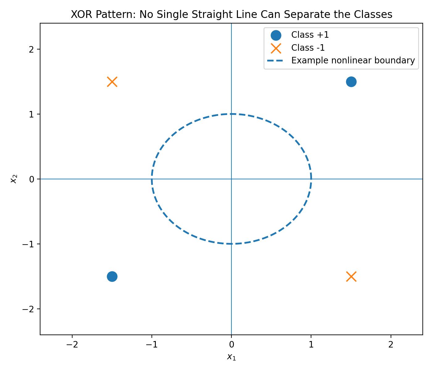XOR pattern that cannot be separated by one line

---

14.2 It May Not Converge on Non-Separable Data

Real data may contain:

• sensor noise
• incorrect labels
• overlapping classes
• missing important features

If perfect separation is impossible, the Perceptron may continue changing its weights without reaching zero training error.

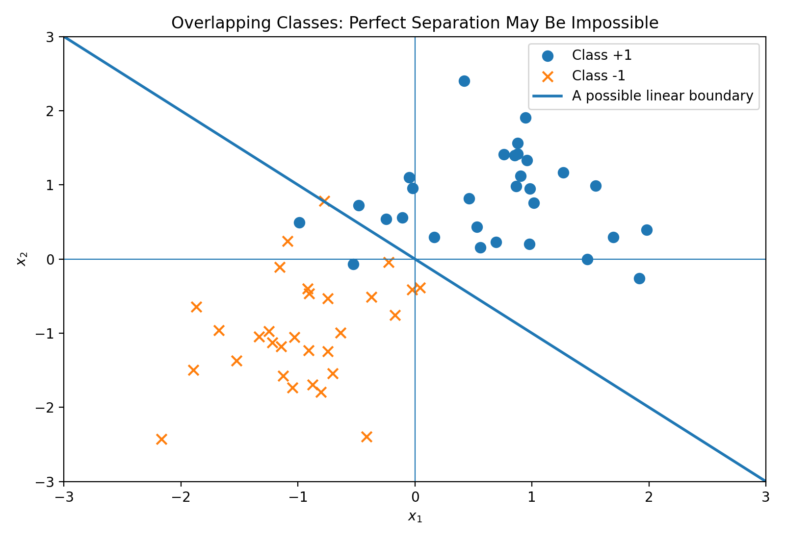Overlapping classes that cannot be perfectly separated

Practical implementations therefore use a maximum number of epochs or another stopping condition.

---

14.3 It Does Not Necessarily Find the Best Boundary

Many different lines may correctly separate the training data.

The Perceptron finds one of them, but not necessarily the most stable one.

The result may depend on:

• training-example order
• initial weights
• learning rate
• number of epochs

A boundary with a larger margin is usually less sensitive to small changes in the input.

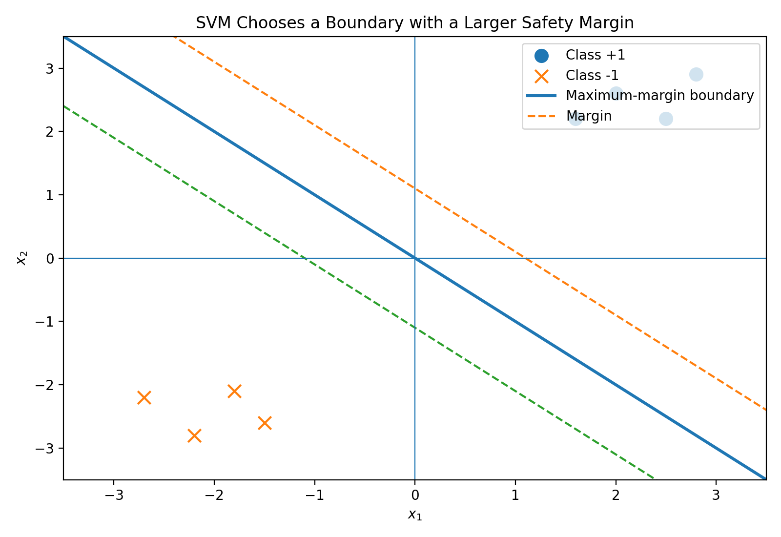Maximum-margin boundary

---

14.4 It Does Not Produce Probabilities

The Perceptron predicts only:

$$+1$$

or:

$$-1$$

A score of $0.01$ and a score of $100$ both produce the same positive prediction.

The score is not a probability.

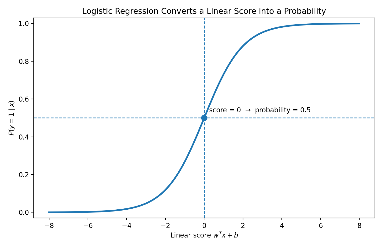Sigmoid function used by Logistic Regression

---

14.5 It Is Sensitive to Feature Scale

Suppose the features are:

• temperature measured from 0 to 100
• vibration measured from 0 to 2

Temperature may dominate the dot product simply because it uses larger numbers.

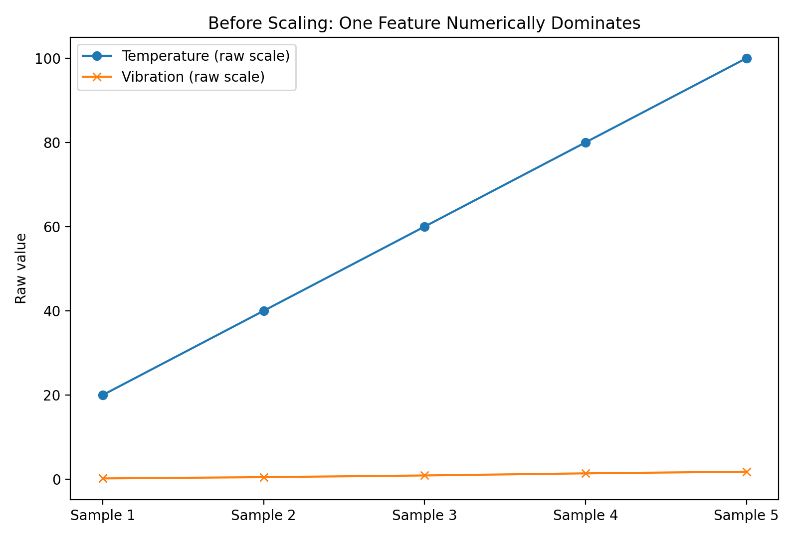Features before scaling

After standardization, both features use comparable scales.

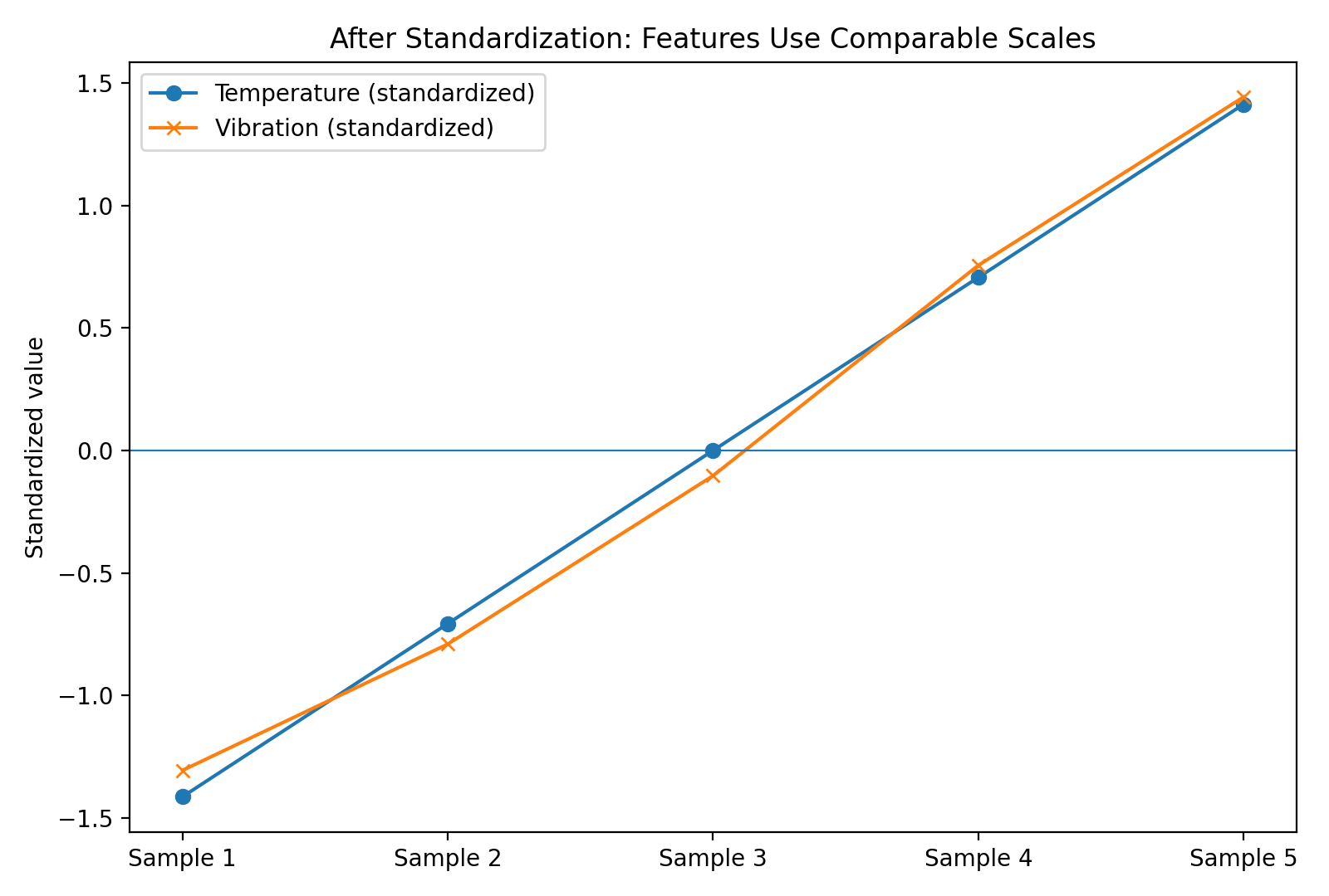Features after standardization

---

15. How Later Methods Address These Limitations

The rows below follow the same order as the limitations in Section 14.

These methods will be studied later. For now, the important idea is that each one addresses a specific weakness of the basic Perceptron.

---

16. Using scikit-learn

import pandas as pd

from sklearn.linear_model import Perceptron
from sklearn.metrics import accuracy_score
from sklearn.model_selection import train_test_split
from sklearn.pipeline import Pipeline
from sklearn.preprocessing import StandardScaler


RANDOM_STATE = 2026

FEATURE_COLUMNS = [
    "temperature_deviation",
    "vibration_deviation",
]

NORMAL_LABEL = 0
ALARM_LABEL = 1


def create_dataset() -> tuple[pd.DataFrame, pd.Series]:
    """Create the example machine-monitoring dataset."""

    X = pd.DataFrame(
        [
            [2.0, 1.0],
            [1.5, 1.8],
            [2.5, 0.5],
            [0.8, 2.2],
            [1.2, 1.0],
            [2.2, 1.5],
            [0.5, 1.6],
            [1.8, 0.7],
            [-1.0, -1.5],
            [-1.8, -0.8],
            [-2.2, -1.7],
            [-0.7, -2.0],
            [-1.5, -1.3],
            [-2.3, -0.5],
            [-0.6, -1.1],
            [-1.2, -0.7],
        ],
        columns=FEATURE_COLUMNS,
    )

    y = pd.Series(
        [
            ALARM_LABEL,
            ALARM_LABEL,
            ALARM_LABEL,
            ALARM_LABEL,
            ALARM_LABEL,
            ALARM_LABEL,
            ALARM_LABEL,
            ALARM_LABEL,
            NORMAL_LABEL,
            NORMAL_LABEL,
            NORMAL_LABEL,
            NORMAL_LABEL,
            NORMAL_LABEL,
            NORMAL_LABEL,
            NORMAL_LABEL,
            NORMAL_LABEL,
        ],
        name="machine_status",
    )

    return X, y


def build_model() -> Pipeline:
    """Build the preprocessing and classification pipeline."""

    return Pipeline(
        steps=[
            (
                "scaler",
                StandardScaler(),
            ),
            (
                "classifier",
                Perceptron(
                    max_iter=1000,
                    eta0=1.0,
                    tol=1e-3,
                    random_state=RANDOM_STATE,
                ),
            ),
        ]
    )


def main() -> None:
    X, y = create_dataset()

    X_train, X_test, y_train, y_test = train_test_split(
        X,
        y,
        test_size=0.25,
        random_state=RANDOM_STATE,
        stratify=y,
    )

    model = build_model()

    # Train the complete pipeline:
    # StandardScaler.fit_transform() followed by Perceptron.fit()
    model.fit(X_train, y_train)

    # Evaluate the model
    training_predictions = model.predict(X_train)
    test_predictions = model.predict(X_test)

    training_accuracy = accuracy_score(
        y_train,
        training_predictions,
    )

    test_accuracy = accuracy_score(
        y_test,
        test_predictions,
    )

    print(f"Training accuracy: {training_accuracy:.2f}")
    print(f"Test accuracy: {test_accuracy:.2f}")

    # Predict a new machine status
    new_machine = pd.DataFrame(
        [
            {
                "temperature_deviation": 1.4,
                "vibration_deviation": 0.9,
            }
        ]
    )

    prediction = model.predict(new_machine)[0]
    decision_score = model.decision_function(new_machine)[0]

    print(f"Decision score: {decision_score:.2f}")

    if prediction == ALARM_LABEL:
        print("Prediction: Alarm")
    else:
        print("Prediction: Normal")


if __name__ == "__main__":
    main()

16.1 Loading the Downloadable CSV

The complete example above keeps the dataset inside create_dataset(), so it can be copied and run as one self-contained script.

Alternatively, download machine_monitoring_dataset.csv and replace the call to create_dataset() with:

dataset = pd.read_csv("machine_monitoring_dataset.csv")

X = dataset[FEATURE_COLUMNS]
y = dataset["machine_status"]

Both options use the same 16 observations and labels. The remaining preprocessing, training, evaluation, and prediction code stays unchanged.

---

17. Connecting the Code to the Mathematics

The decision score is conceptually:

$$w^Tx+b$$

• positive score: predict the positive class
• negative score: predict the negative class
• score near zero: close to the decision boundary

The decision score is not a probability.

---

18. Key Takeaways

Prediction

$$\hat y=\operatorname{sign}(w^Tx+b)$$

Mistake condition

$$y_i(w^Tx_i+b)\leq0$$

Update

$$w\leftarrow w+\eta y_ix_i$$ $$b\leftarrow b+\eta y_i$$

Convergence

If the data is linearly separable, the Perceptron will find a separating boundary after a finite number of mistakes.

Main limitation

A single Perceptron can only learn a linear decision boundary.