Logistic Regression: Turning Linear Scores into Probabilities

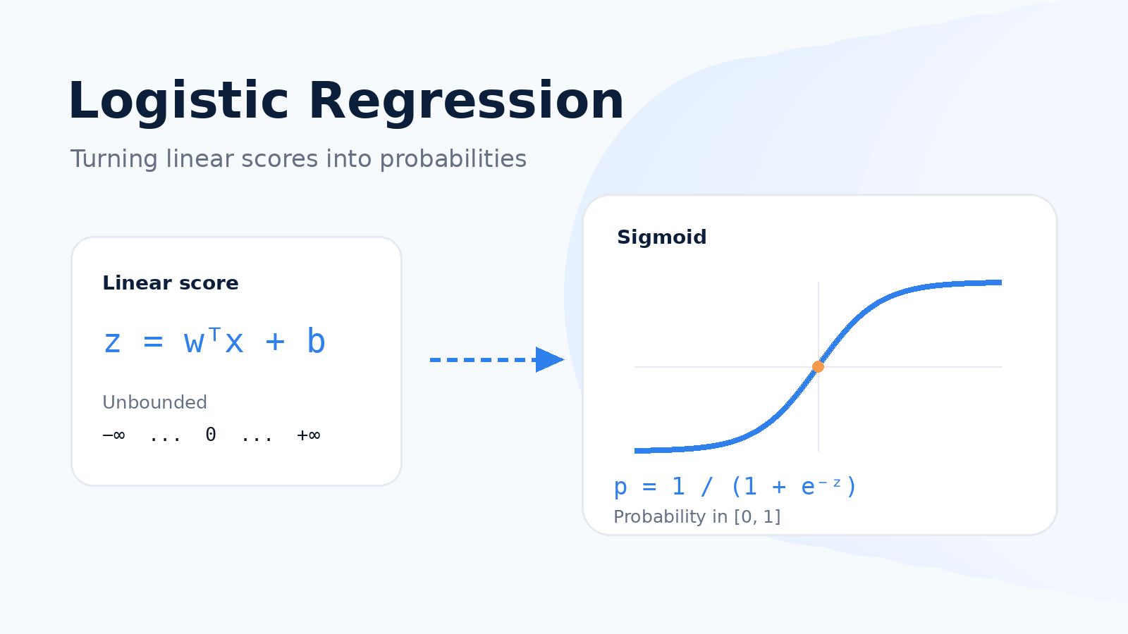A linear score transformed into a probability by the sigmoid function

Learning Objectives

By the end of this lesson, you should be able to:

1. Explain why a Perceptron decision score is not a probability.
2. Convert a linear score into an estimated class probability with the sigmoid function.
3. Interpret Logistic Regression through probability, odds, and log-odds.
4. Make a complete binary prediction by hand.
5. Explain why maximum likelihood leads to binary cross-entropy.
6. Interpret the gradient update $w \leftarrow w-\eta(p-y)x$.
7. Extend binary Logistic Regression to multiple classes with softmax.
8. Train and evaluate Logistic Regression with a leakage-safe scikit-learn pipeline.

---

1. The Problem: A Class Label Is Not Enough

Suppose a factory monitors a machine using two sensors:

• $x_1$: temperature deviation from its normal operating level
• $x_2$: vibration deviation from its normal operating level

The target is:

$$y= \begin{cases} 1 & \text{an alarm-worthy event occurs within one hour}\\ 0 & \text{the machine remains normal} \end{cases}$$

A binary classifier can predict alarm or normal, but an operations team often needs more information.

A hard label treats Machines B and C the same if both fall on the alarm side of the decision boundary. A probability is more useful because it supports actions such as:

• inspecting the highest-risk machines first
• selecting a threshold based on the cost of false alarms
• combining model output with maintenance capacity

The desired model output is therefore:

$$P(y=1\mid x)$$

This is the model's estimated probability of an alarm-worthy event for a machine with features $x$.

---

2. The Basic Idea: Keep the Score, Replace the Hard Threshold

A Perceptron begins with the linear score:

$$z=w^Tx+b$$

and immediately converts it into a class using its sign.

A score of $0.2$ and a score of $4.0$ both produce the positive class. The score magnitude may indicate distance from the boundary, but it is:

• unbounded
• dependent on feature scale and learned weights
• not directly interpretable as a probability

Logistic Regression keeps the same linear score but passes it through a smooth function:

$$z=w^Tx+b \quad\longrightarrow\quad p=\sigma(z)$$

where $p=P(y=1\mid x)$.

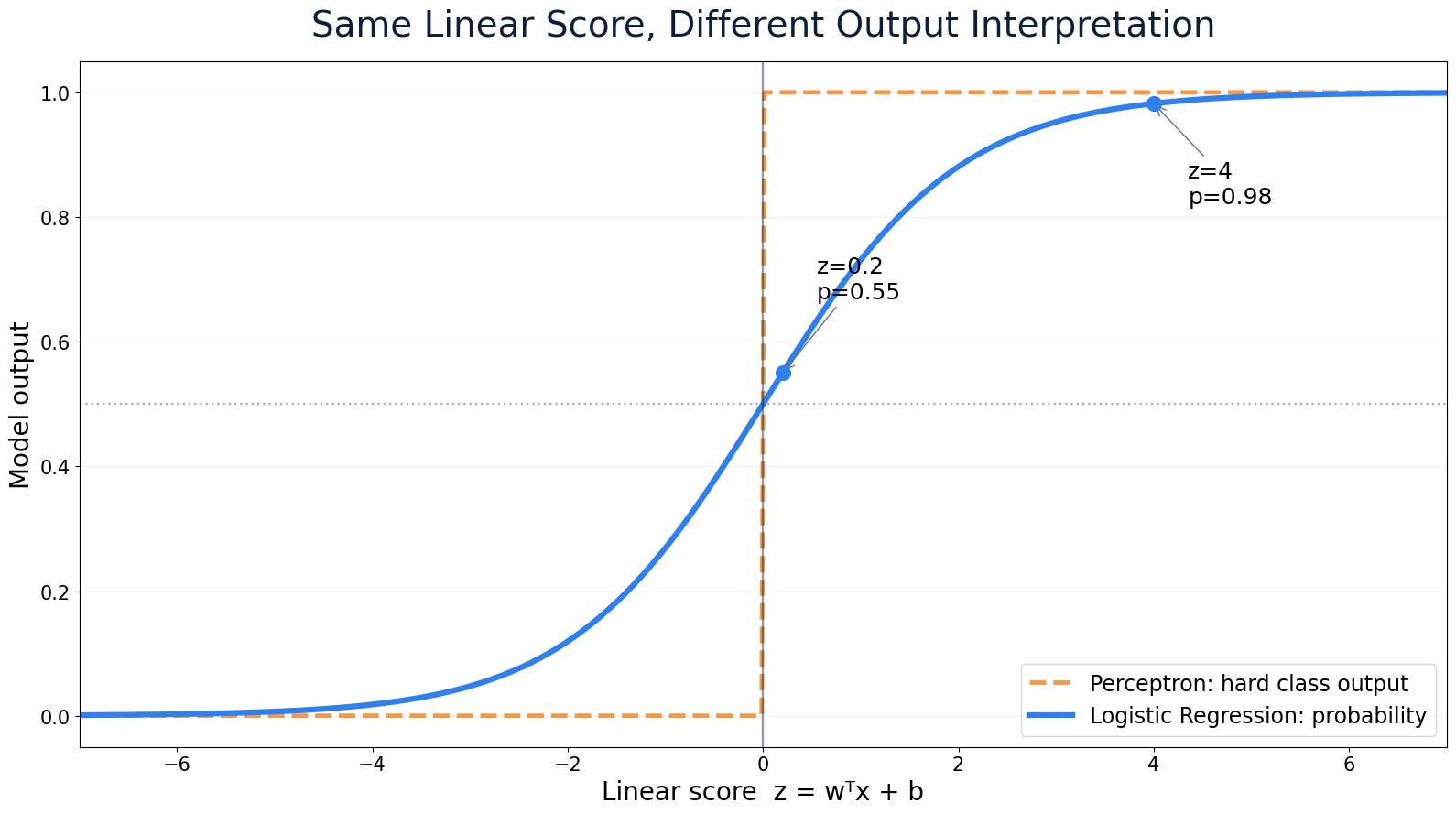Comparison of a hard Perceptron output and a Logistic Regression probability

The important change is not only that the output lies between 0 and 1. Logistic Regression also defines a Bernoulli probability model and learns its parameters by maximizing the probability of the observed labels.

A value such as $p=0.80$ means the model assigns an 80% probability to class 1. It does not automatically guarantee that the model is correct 80% of the time; that requires calibration to be checked on representative data.

---

3. The Main Formula

Logistic Regression uses two connected formulas.

3.1 Linear score

$$z=w^Tx+b$$

where:

• $x\in\mathbb{R}^d$ is the feature vector
• $w\in\mathbb{R}^d$ is the weight vector
• $b\in\mathbb{R}$ is the bias
• $z\in\mathbb{R}$ is the raw decision score

For two machine-monitoring features:

$$z=w_1x_1+w_2x_2+b$$

Each weight controls how strongly its feature changes the score.

3.2 Sigmoid transformation

$$p=\sigma(z)=\frac{1}{1+e^{-z}}$$

where:

• $p=P(y=1\mid x)$
• $1-p=P(y=0\mid x)$
• $e$ is the base of the natural logarithm

The sigmoid is monotone: a larger score always produces a larger probability.

For example, if:

$$z=1.2$$

then:

$$p=\frac{1}{1+e^{-1.2}}\approx0.7685$$

The model therefore assigns approximately a 76.9% probability to an alarm.

Limitation of the formula: the model assumes that the log-odds, not necessarily the probability itself, changes linearly with the features.

---

4. Why Is the Formula Designed This Way?

4.1 Why not use the score directly as a probability?

A first attempt might be:

$$p=w^Tx+b$$

This fails because a probability must lie in $[0,1]$, while a linear score can be any real number.

4.2 Model the log-odds as a linear function

For a probability $p$, the odds of class 1 are:

$$\frac{p}{1-p}$$

The log-odds, also called the logit, are:

$$\log\left(\frac{p}{1-p}\right)$$

Log-odds can range from $-\infty$ to $+\infty$, so they can be matched naturally with a linear score:

$$\log\left(\frac{p}{1-p}\right)=w^Tx+b=z$$

Solving this equation for $p$ gives the sigmoid:

$$\frac{p}{1-p}=e^z$$ $$p=e^z(1-p)$$ $$p(1+e^z)=e^z$$ $$p=\frac{e^z}{1+e^z}=\frac{1}{1+e^{-z}}$$

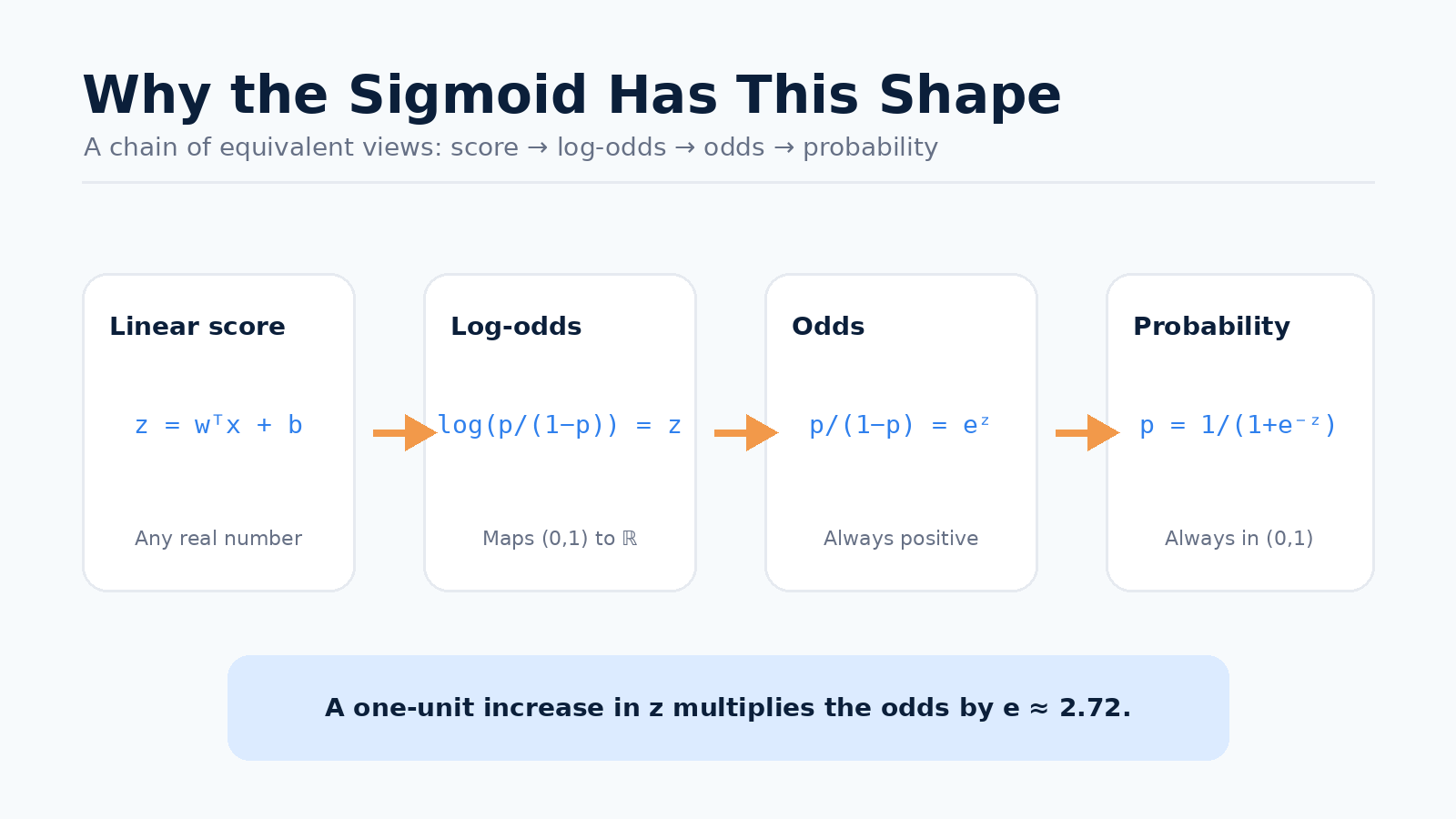Mapping from a linear score to log-odds, odds, and probability

This construction has three useful properties:

1. Every real-valued score becomes a valid probability.
2. The transformation is monotone, so score ordering is preserved.
3. A one-unit increase in the score multiplies the odds by $e\approx2.72$.

4.3 The decision boundary stays linear

Because:

$$\sigma(0)=0.5$$

we have:

$$p\geq0.5 \quad\Longleftrightarrow\quad z\geq0$$

Therefore, with a threshold of 0.5, Logistic Regression and a sign-based linear classifier use the same type of boundary:

$$w^Tx+b=0$$

Logistic Regression does not make the boundary nonlinear. It adds a probability surface around that boundary.

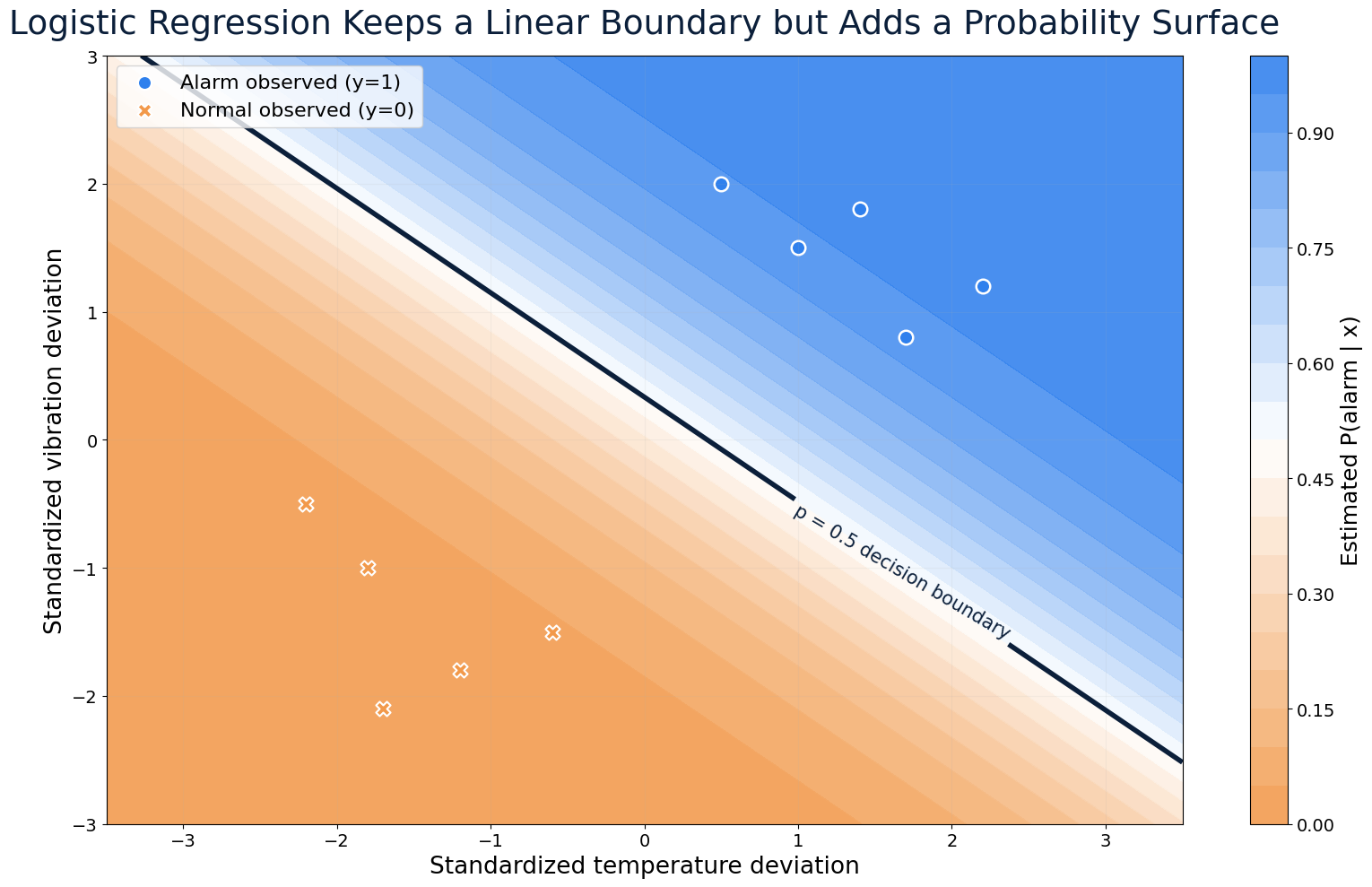A Logistic Regression probability surface with a linear decision boundary

---

5. Prediction Process

Assume the features have already been standardized and the learned model is:

$$w= \begin{bmatrix} 1.2\\ 0.8 \end{bmatrix}, \qquad b=-0.4$$

A new machine has:

$$x= \begin{bmatrix} 1.0\\ 0.5 \end{bmatrix}$$

Step 1: Calculate the linear score

$$z=w^Tx+b$$ $$z=(1.2)(1.0)+(0.8)(0.5)-0.4$$ $$z=1.2+0.4-0.4=1.2$$

Step 2: Convert the score into a probability

$$p=\sigma(1.2)=\frac{1}{1+e^{-1.2}}\approx0.7685$$

The equivalent odds are:

$$\frac{p}{1-p}=e^{1.2}\approx3.32$$

The model estimates that an alarm is about 3.32 times as likely as no alarm for this machine.

Step 3: Apply a decision threshold

Using the common threshold $0.5$:

$$0.7685\geq0.5$$

so:

$$\hat y=1$$

The machine is predicted to trigger an alarm.

The threshold is an operational choice. If automatic shutdown requires $p\geq0.80$, the same machine would not yet be shut down automatically, even though its most likely class remains alarm.

---

6. How the Model Learns

The model must choose $w$ and $b$ so that observed positive examples receive high probabilities and observed negative examples receive low probabilities.

6.1 Bernoulli likelihood for one example

For one example $(x_i,y_i)$, let:

$$p_i=\sigma(w^Tx_i+b)$$

The probability assigned to the observed label can be written compactly as:

$$P(y_i\mid x_i,w,b) = p_i^{y_i}(1-p_i)^{1-y_i}$$

This works because $y_i$ is either 0 or 1.

• If $y_i=1$, the expression becomes $p_i$.
• If $y_i=0$, the expression becomes $1-p_i$.

6.2 Maximum likelihood

For independent training examples, the likelihood is:

$$\mathcal{L}(w,b) = \prod_{i=1}^{n} p_i^{y_i}(1-p_i)^{1-y_i}$$

Training chooses parameters that maximize this likelihood.

Products of many probabilities are inconvenient numerically, so we take logarithms and minimize the negative average log-likelihood:

$$J(w,b) = -\frac{1}{n} \sum_{i=1}^{n} \left[ y_i\log p_i+(1-y_i)\log(1-p_i) \right]$$

This is binary cross-entropy, also called log loss.

For one example:

$$\ell_i = -\left[ y_i\log p_i+(1-y_i)\log(1-p_i) \right]$$

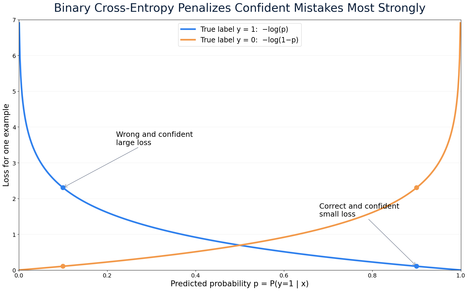Binary cross-entropy loss for positive and negative examples

Cross-entropy is designed so that:

• a correct, confident prediction has small loss
• an uncertain prediction has moderate loss
• a wrong, confident prediction has very large loss

6.3 The optimization loop

There is no general closed-form formula for the optimal Logistic Regression coefficients. A numerical optimizer therefore repeats:

1. Initialize $w$ and $b$.
2. Compute scores $z_i$.
3. Convert scores to probabilities $p_i$.
4. Compute loss and gradients.
5. Update the parameters.
6. Stop when improvement is sufficiently small or a maximum iteration count is reached.

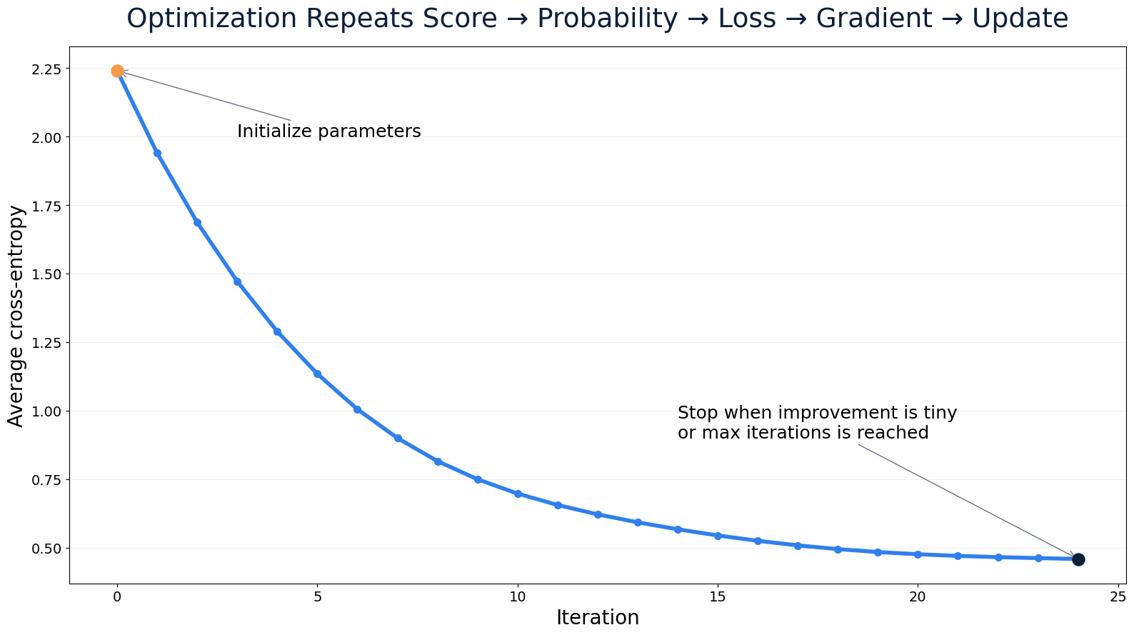Illustrative optimization process for Logistic Regression

Optimization methods such as gradient descent, stochastic gradient descent, quasi-Newton methods, and Newton-style methods differ mainly in how they choose the update direction and step size. Their detailed mechanics are not required here.

Practical implementations commonly add regularization:

$$J_{\text{regularized}}(w,b) = J(w,b)+\frac{\lambda}{2}\lVert w\rVert^2$$

Regularization discourages excessively large coefficients and gives a finite, more stable solution in many difficult datasets.

---

7. Why the Gradient Update Works

For one training example, the cross-entropy gradients simplify to:

$$\nabla_w\ell=(p-y)x$$ $$\frac{\partial\ell}{\partial b}=p-y$$

A gradient-descent step is:

$$w\leftarrow w-\eta(p-y)x$$ $$b\leftarrow b-\eta(p-y)$$

where $\eta>0$ is the learning rate.

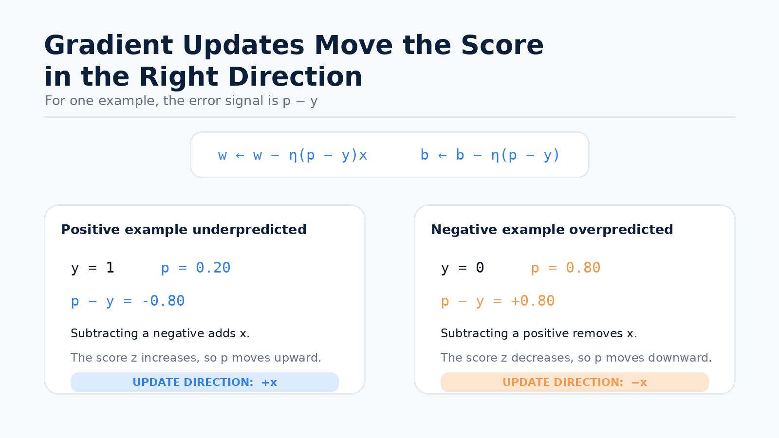Gradient update intuition for positive and negative examples

7.1 A positive example receives too small a probability

Suppose:

$$y=1, \qquad p=0.20$$

Then:

$$p-y=-0.80$$

The update becomes:

$$w\leftarrow w+0.80\eta x$$

The model adds the example's direction to the weight vector, increasing its future score and probability.

7.2 A negative example receives too large a probability

Suppose:

$$y=0, \qquad p=0.80$$

Then:

$$p-y=0.80$$

The update becomes:

$$w\leftarrow w-0.80\eta x$$

The model moves against the example's direction, decreasing its future score and probability.

7.3 Compact mathematical argument

For the current example, update both $w$ and $b$:

$$w_{\text{new}}=w-\eta(p-y)x$$ $$b_{\text{new}}=b-\eta(p-y)$$

Its new score is:

$$z_{\text{new}} = w_{\text{new}}^Tx+b_{\text{new}}$$ $$z_{\text{new}} = z-\eta(p-y)(\lVert x\rVert^2+1)$$

• If $y=1$, then $p-y<0$, so $z_{\text{new}}>z$.
• If $y=0$, then $p-y>0$, so $z_{\text{new}}<z$.

The score always moves in the desired direction for the current example. A sufficiently small learning rate is still needed to ensure stable loss reduction across the full dataset.

---

8. Manual Walkthrough

Use two standardized training examples and stochastic gradient descent:

$$x_1= \begin{bmatrix} 2\\ 1 \end{bmatrix}, \quad y_1=1$$ $$x_2= \begin{bmatrix} -1\\ -2 \end{bmatrix}, \quad y_2=0$$

Initialize:

$$w= \begin{bmatrix} 0\\ 0 \end{bmatrix}, \qquad b=0, \qquad \eta=0.2$$

8.1 First example: positive label

Current score and probability:

$$z_1=0, \qquad p_1=\sigma(0)=0.5$$

Error signal:

$$p_1-y_1=0.5-1=-0.5$$

Gradients:

$$\nabla_w\ell_1=(-0.5) \begin{bmatrix} 2\\ 1 \end{bmatrix} = \begin{bmatrix} -1\\ -0.5 \end{bmatrix}$$ $$\frac{\partial\ell_1}{\partial b}=-0.5$$

Update:

$$w\leftarrow \begin{bmatrix} 0\\ 0 \end{bmatrix} -0.2 \begin{bmatrix} -1\\ -0.5 \end{bmatrix} = \begin{bmatrix} 0.2\\ 0.1 \end{bmatrix}$$ $$b\leftarrow0-0.2(-0.5)=0.1$$

8.2 Second example: negative label

With the updated parameters:

$$z_2=(0.2)(-1)+(0.1)(-2)+0.1=-0.3$$ $$p_2=\sigma(-0.3)\approx0.4256$$

Error signal:

$$p_2-y_2=0.4256-0=0.4256$$

Gradients:

$$\nabla_w\ell_2 = 0.4256 \begin{bmatrix} -1\\ -2 \end{bmatrix} = \begin{bmatrix} -0.4256\\ -0.8511 \end{bmatrix}$$ $$\frac{\partial\ell_2}{\partial b}=0.4256$$

Update:

$$w\leftarrow \begin{bmatrix} 0.2\\ 0.1 \end{bmatrix} -0.2 \begin{bmatrix} -0.4256\\ -0.8511 \end{bmatrix} \approx \begin{bmatrix} 0.2851\\ 0.2702 \end{bmatrix}$$ $$b\leftarrow0.1-0.2(0.4256)\approx0.0149$$

The weights increased numerically because the negative example has negative feature values. This still lowers that example's score: a positive weight multiplied by a negative feature contributes a negative amount.

---

9. Complete Algorithm

Input:
    training examples (x_i, y_i), with y_i in {0, 1}
    learning rate eta
    regularization strength lambda

Initialize weights w
Initialize bias b

Repeat until convergence or maximum iterations:

    For each example i:
        z_i = w^T x_i + b
        p_i = 1 / (1 + exp(-z_i))

    loss = average binary cross-entropy
           + (lambda / 2) * ||w||^2

    gradient_w = average of (p_i - y_i) * x_i
                 + lambda * w
    gradient_b = average of (p_i - y_i)

    w = w - eta * gradient_w
    b = b - eta * gradient_b

For a new x:
    z = w^T x + b
    p = sigmoid(z)
    predict class 1 when p >= chosen threshold

A library optimizer may not follow these exact full-batch steps, but it minimizes the same type of objective.

---

10. Multiclass Logistic Regression

Binary Logistic Regression needs one score because there are only two complementary probabilities:

$$P(y=0\mid x)=1-P(y=1\mid x)$$

For $K$ classes, the model calculates one score per class:

$$z_k=w_k^Tx+b_k$$

It then applies the softmax function:

$$P(y=k\mid x) = \frac{e^{z_k}} {\sum_{j=1}^{K}e^{z_j}}$$

where:

• $z_k$ is the score for class $k$
• all class probabilities are positive
• the probabilities sum to 1
• the predicted class is the one with the largest probability

Suppose a machine can be classified as:

1. normal
2. inspect soon
3. shutdown now

and its class scores are:

$$z= \begin{bmatrix} 1.2\\ 0.4\\ -0.2 \end{bmatrix}$$

For numerical stability, subtract the largest score before exponentiating:

$$z-\max(z)= \begin{bmatrix} 0\\ -0.8\\ -1.4 \end{bmatrix}$$

The resulting probabilities are approximately:

$$P(y\mid x) = \begin{bmatrix} 0.590\\ 0.265\\ 0.145 \end{bmatrix}$$

The model predicts normal, but it still communicates meaningful probability mass for the two intervention classes.

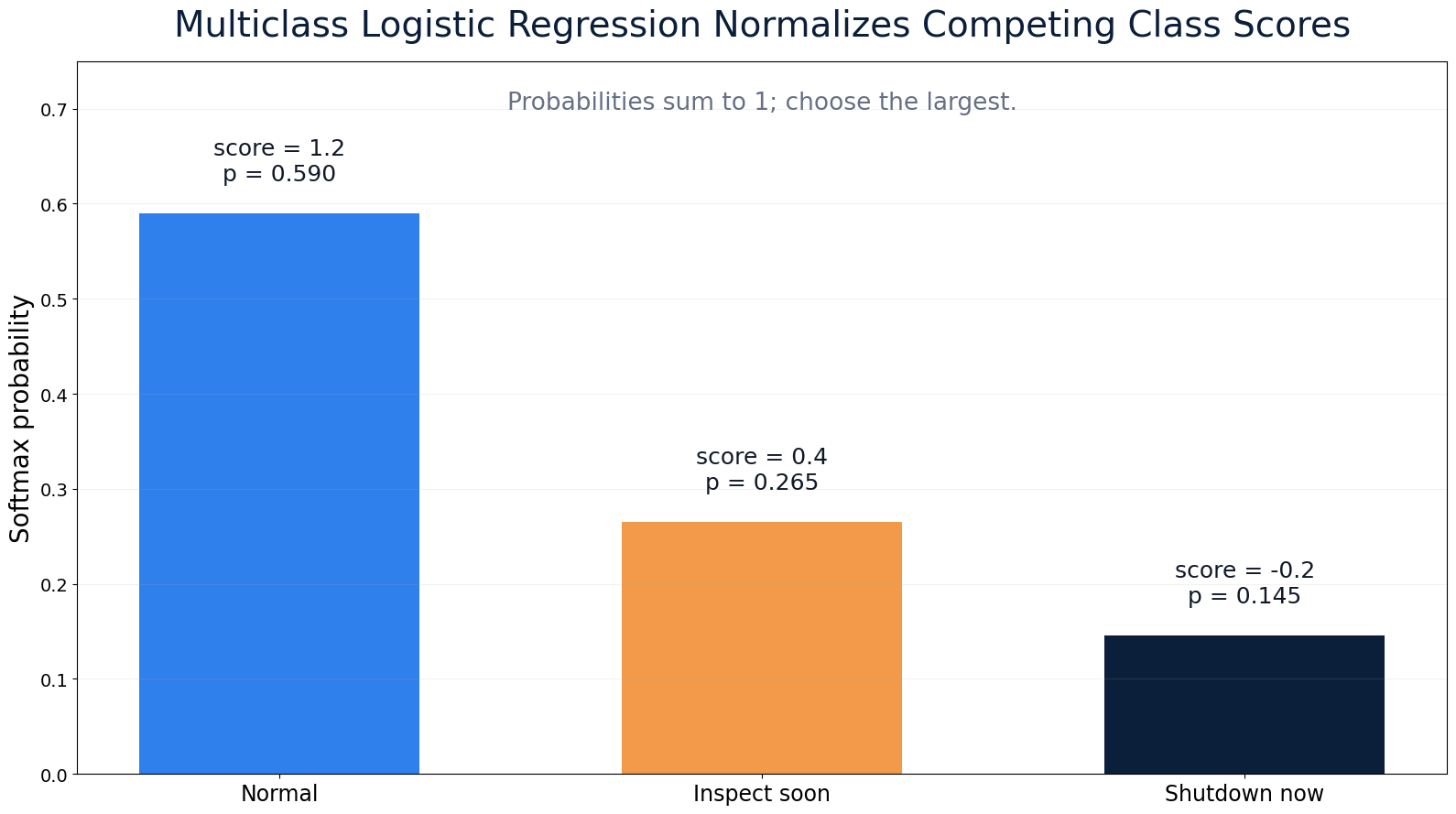Softmax probabilities for three machine states

---

11. When Does It Work?

Logistic Regression is most effective when:

• the log-odds can be approximated by a linear function of the available features
• the training data represents the cases expected during deployment
• labels are defined consistently
• important nonlinear relationships are represented through engineered features or transformations
• regularization is used when data is limited, correlated, or nearly separable
• probability quality and the decision threshold are validated on held-out data

What is guaranteed mathematically?

For standard linear Logistic Regression, binary cross-entropy is a convex function of the parameters. With a convex regularizer such as L2 regularization, the complete objective remains convex.

Therefore:

• there are no inferior local minima
• a converged optimizer reaches a global minimum of the stated objective

This does not guarantee:

• low error on unseen data
• well-calibrated probabilities
• robustness to distribution shift
• a nonlinear decision boundary

Logistic Regression can train on overlapping, non-separable classes because it minimizes total loss rather than demanding zero classification mistakes. However, perfectly separable data creates a different issue: without regularization, the likelihood can keep improving as coefficient magnitudes grow without bound.

---

12. Limitations

12.1 It still has a linear decision boundary

The boundary remains:

$$w^Tx+b=0$$

The sigmoid changes the output interpretation, not the boundary shape. Nonlinear patterns require transformed features or a nonlinear model.

12.2 Perfect separation can make the unregularized solution diverge

If one linear boundary perfectly separates all labels, unregularized maximum likelihood may not have a finite coefficient solution. Increasing the coefficient magnitudes can keep pushing probabilities closer to 0 and 1.

12.3 A probability output is not automatically calibrated

A model may output $0.8$ without events occurring 80% of the time among similar predictions. Misspecified features, sampling bias, class imbalance, and distribution shift can damage calibration.

12.4 Coefficients can be unstable with correlated features or influential observations

When features carry nearly the same information, many coefficient combinations can produce similar predictions. Extreme observations can also exert strong influence on the fitted boundary.

12.5 Feature scale affects optimization and regularization

A feature measured in large units can receive a numerically small coefficient while an equivalent standardized feature receives a larger one. Scaling also affects how regularization penalizes different coefficients and how quickly numerical solvers converge.

---

13. How Later Methods Address the Limitations

These are previews rather than complete treatments. The central point is that Logistic Regression solves the Perceptron's missing-probability problem, but it does not solve every limitation of a linear model.

---

14. Practical Implementation

The following scikit-learn example creates an overlapping machine-monitoring dataset, splits it before preprocessing, standardizes the features inside a Pipeline, trains a regularized Logistic Regression model, evaluates both labels and probabilities, and predicts one new machine state.

from __future__ import annotations

import numpy as np
import pandas as pd
from sklearn.linear_model import LogisticRegression
from sklearn.metrics import accuracy_score, log_loss
from sklearn.model_selection import train_test_split
from sklearn.pipeline import Pipeline
from sklearn.preprocessing import StandardScaler

RANDOM_STATE = 42
TEST_SIZE = 0.25
N_SAMPLES = 240

FEATURE_COLUMNS = [
    "temperature_deviation_c",
    "vibration_deviation_mm_s",
]

NORMAL_LABEL = 0
ALARM_LABEL = 1


def sigmoid(score: np.ndarray) -> np.ndarray:
    """Convert linear scores into probabilities."""
    return 1.0 / (1.0 + np.exp(-score))


def create_dataset() -> tuple[pd.DataFrame, pd.Series]:
    """Create a reproducible machine-monitoring dataset."""
    rng = np.random.default_rng(RANDOM_STATE)

    temperature = rng.normal(loc=0.8, scale=1.4, size=N_SAMPLES)
    vibration = rng.normal(loc=0.4, scale=0.9, size=N_SAMPLES)

    hidden_score = 0.9 * temperature + 1.3 * vibration - 0.9
    alarm_probability = sigmoid(hidden_score)
    labels = rng.binomial(n=1, p=alarm_probability)

    X = pd.DataFrame(
        {
            FEATURE_COLUMNS[0]: temperature,
            FEATURE_COLUMNS[1]: vibration,
        }
    )
    y = pd.Series(labels, name="alarm_within_one_hour")
    return X, y


def build_model() -> Pipeline:
    """Build preprocessing and Logistic Regression in one pipeline."""
    return Pipeline(
        steps=[
            ("scaler", StandardScaler()),
            (
                "classifier",
                LogisticRegression(
                    C=1.0,
                    solver="lbfgs",
                    max_iter=1000,
                ),
            ),
        ]
    )


def positive_class_index(model: Pipeline) -> int:
    """Find the probability column for the alarm label."""
    classifier = model.named_steps["classifier"]
    return int(np.flatnonzero(classifier.classes_ == ALARM_LABEL)[0])


def main() -> None:
    X, y = create_dataset()

    X_train, X_test, y_train, y_test = train_test_split(
        X,
        y,
        test_size=TEST_SIZE,
        random_state=RANDOM_STATE,
        stratify=y,
    )

    model = build_model()
    model.fit(X_train, y_train)

    train_predictions = model.predict(X_train)
    test_predictions = model.predict(X_test)
    alarm_index = positive_class_index(model)
    test_probabilities = model.predict_proba(X_test)[:, alarm_index]

    train_accuracy = accuracy_score(y_train, train_predictions)
    test_accuracy = accuracy_score(y_test, test_predictions)
    test_cross_entropy = log_loss(
        y_test,
        test_probabilities,
        labels=[0, 1],
    )

    print(f"Training accuracy: {train_accuracy:.3f}")
    print(f"Test accuracy: {test_accuracy:.3f}")
    print(f"Test cross-entropy: {test_cross_entropy:.3f}")

    new_machine = pd.DataFrame(
        [
            {
                "temperature_deviation_c": 1.6,
                "vibration_deviation_mm_s": 0.9,
            }
        ]
    )

    raw_score = float(model.decision_function(new_machine)[0])
    alarm_probability = float(
        model.predict_proba(new_machine)[0, alarm_index]
    )
    prediction = int(model.predict(new_machine)[0])

    print(f"Raw decision score (log-odds): {raw_score:.3f}")
    print(f"Estimated alarm probability: {alarm_probability:.3f}")
    print(
        "Prediction:",
        "Alarm" if prediction == ALARM_LABEL else "Normal",
    )


if __name__ == "__main__":
    main()

One deterministic run produces:

Training accuracy: 0.711
Test accuracy: 0.833
Test cross-entropy: 0.418
Raw decision score (log-odds): 1.631
Estimated alarm probability: 0.836
Prediction: Alarm

This small synthetic result demonstrates the workflow; it is not evidence that the model would perform well on a real factory deployment.

Connecting the code to the mathematics

The Pipeline fits the scaler using only the training partition and applies the same transformation to test and future observations. This prevents preprocessing information from leaking from the test set into training.

For a binary classifier, predict_proba() returns one column per class in the order stored in classifier.classes_. The code explicitly locates the column for the alarm label rather than assuming a column position.

---

15. Key Takeaways

Prediction rule

$$z=w^Tx+b$$ $$p=P(y=1\mid x)=\frac{1}{1+e^{-z}}$$

Logistic Regression keeps a linear score and converts it into an estimated probability.

Probability interpretation

$$\log\left(\frac{p}{1-p}\right)=w^Tx+b$$

The model is linear in the log-odds. With a threshold of 0.5, its decision boundary is still $w^Tx+b=0$.

Learning objective

$$-\left[y\log p+(1-y)\log(1-p)\right]$$

Binary cross-entropy is the negative log-likelihood of the Bernoulli model and strongly penalizes confident mistakes.

Update rule

$$w\leftarrow w-\eta(p-y)x$$

• If the probability is too low for a positive example, the score is pushed upward.
• If the probability is too high for a negative example, the score is pushed downward.

Multiclass extension

$$P(y=k\mid x)=\frac{e^{z_k}}{\sum_j e^{z_j}}$$

Softmax converts one score per class into probabilities that sum to 1.

Main limitation

Logistic Regression remains a linear classifier in the chosen feature space. Its probabilities are useful model estimates, but their calibration and reliability must be validated on representative data.

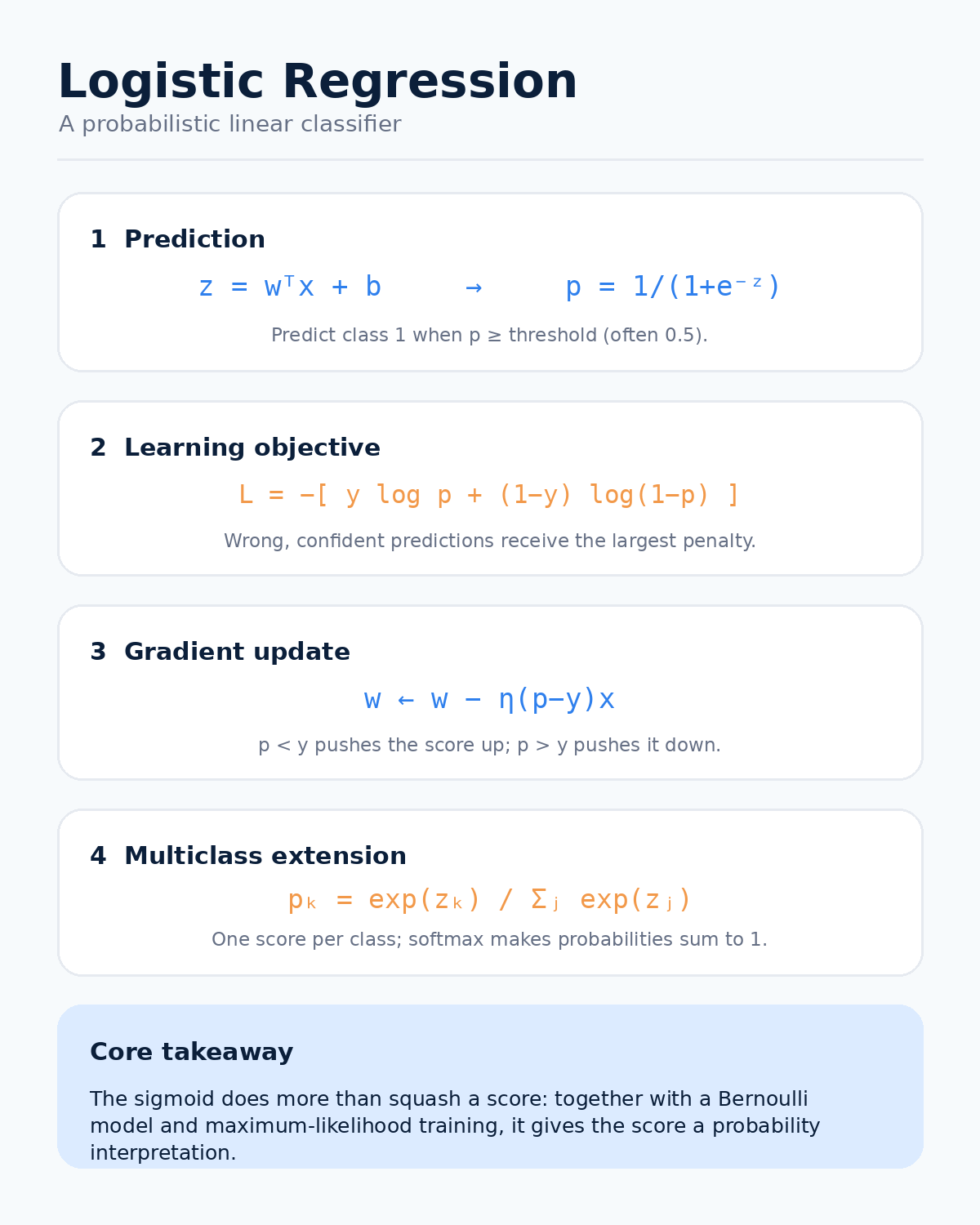Summary infographic for Logistic Regression

---

Reference Notes

• Mathematical topics align with the Bernoulli model, logit parameterization, sigmoid function, maximum likelihood, cross-entropy, iterative optimization, and softmax formulation used in the course materials.
• The implementation follows the stable scikit-learn LogisticRegression, Pipeline, StandardScaler, train_test_split, predict_proba, and log_loss APIs checked in July 2026.