topic: Machine Learning Algorithms
Linear Regression: From Fitting a Line to Regularized Models
Build Linear Regression from simple and multiple prediction through residual loss, model limitations, Lasso and Ridge regularization, and leakage-safe cross-validation.
Table of contents
 Linear regression from a best-fit line to regularized models
This lesson begins a broader progression through machine learning: from supervised to unsupervised learning, from linear to nonlinear models, and from classical statistical methods to deep learning. Linear regression is a useful starting point because its prediction rule, loss function, assumptions, and limitations can all be inspected directly.
This lesson focuses on the practical workflow: how linear regression predicts, how loss guides fitting, how the model extends to multiple features, where ordinary linear regression becomes unreliable, and how regularization and cross-validation address specific weaknesses.
Learning Objectives
By the end of this lesson, you should be able to:
- Explain what simple and multiple linear regression are trying to predict.
- Interpret the intercept, coefficients, predictions, residuals, and squared-error loss.
- Compare candidate regression lines using mean squared error.
- Train simple and multiple linear regression models with scikit-learn.
- Explain the main practical weaknesses of ordinary linear regression.
- Distinguish Lasso regression from Ridge regression.
- Explain why the regularization strength is a hyperparameter.
- Select a Lasso or Ridge penalty with leakage-safe cross-validation.
1. The Prediction Problem
Suppose a factory wants to predict the daily energy consumption of a machine before the day is complete.
For the first model, the factory records only one feature:
operating_hours: how many hours the machine runs during the day
The target is:
energy_kwh: total energy consumed during that day
A small teaching dataset is:
| Machine operating hours | Daily energy use , kWh |
|---|---|
| 4 | 46 |
| 6 | 58 |
| 8 | 68 |
| 10 | 82 |
| 12 | 95 |
| 14 | 104 |
The task is a regression problem because the model predicts a numeric quantity rather than a class label.
The points show a clear pattern: days with more operating hours usually consume more energy, but the observations do not fall perfectly on one line.
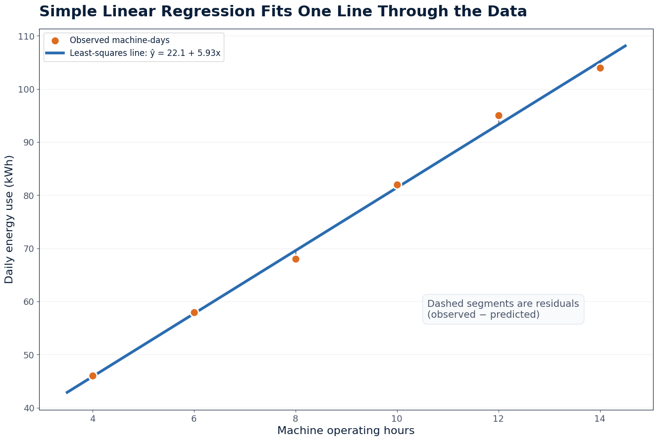 Machine operating hours plotted against daily energy use
The model is not trying to memorize every point. It is trying to learn a compact rule that captures the main relationship and can be applied to a future machine-day.
2. The Basic Idea of Simple Linear Regression
Simple linear regression uses one feature and predicts with a straight line:
where:
- is the input feature, machine operating hours
- is the predicted daily energy use
- is the intercept
- is the slope or weight
In plain language:
Start with a baseline energy value, then add a fixed amount for every additional operating hour.
For example, consider:
For a machine operating for 10 hours:
The coefficient says that the model associates one additional operating hour with an increase of about kWh.
The intercept is the model's predicted energy use when . It is mathematically necessary for positioning the line, but it is only physically meaningful when zero operating hours is a realistic value within the relevant data range.
Why a line?
A line is the simplest rule that can represent a constant rate of change. It is easy to fit, fast to evaluate, and directly interpretable.
Its limitation is equally important: one straight line cannot represent a relationship whose slope changes substantially across the input range.
3. Prediction Error and Loss
For observation , the model makes prediction:
The residual is:
where:
- is the observed energy use
- is the predicted energy use
- is the signed prediction error
A positive residual means the model predicted too low. A negative residual means it predicted too high.
For the 10-hour observation:
so:
For the 14-hour observation:
so:
To evaluate an entire line, ordinary linear regression squares the residuals and adds them:
The mean squared error is:
Squaring has three effects:
- Positive and negative residuals cannot cancel.
- Larger mistakes receive more weight.
- The objective becomes smooth and mathematically convenient.
The main limitation is that a very large residual receives a very large squared penalty, so outliers can strongly influence the fitted line.
4. Trying Different Weights and Comparing Loss
A linear model is defined by its intercept and slope. Different parameter values create different lines.
For the six machine-days, compare three candidates:
| Candidate | Equation | MSE |
|---|---|---|
| Line A | 41.50 | |
| Line B | 2.14 | |
| Line C | 39.00 |
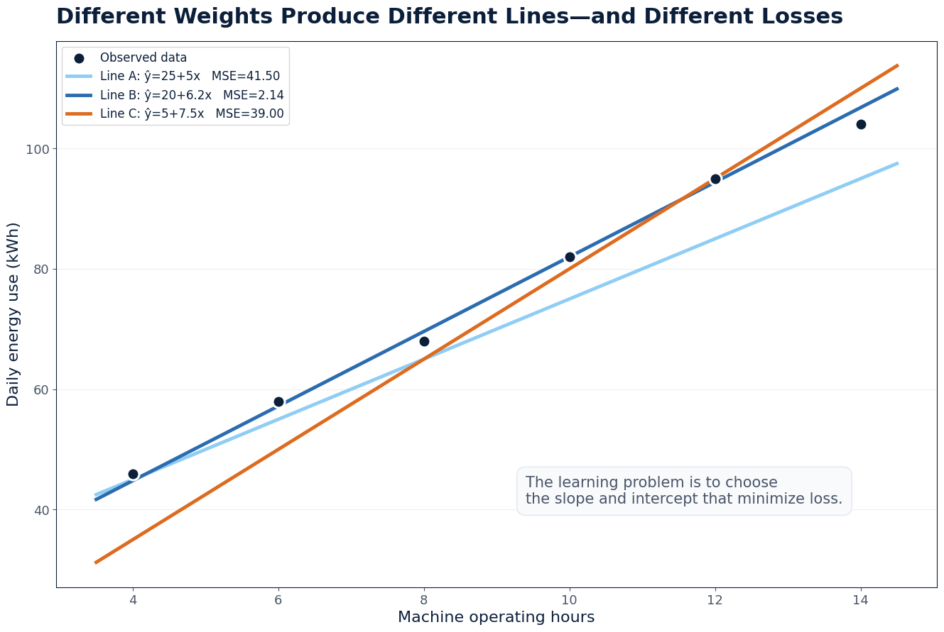 Three candidate regression lines with their mean squared errors
Line B has the smallest MSE among these three candidates, so it fits the observations best among them.
The actual least-squares solution for this dataset is approximately:
Its parameters are not chosen by visual judgment. They are the values that minimize the sum of squared residuals over all possible lines.
What is the model learning?
The learning process is parameter estimation:
The notation means “the parameter values that make the expression as small as possible.”
The fitted coefficients are written with hats because they are estimates learned from a sample, not immutable laws of the physical system.
5. A Complete Numerical Prediction
Using the least-squares line:
suppose a machine will operate for 11 hours.
Substitute :
This is a point prediction. It does not say that the machine must consume exactly 87.37 kWh. Measurement noise, load, ambient temperature, and omitted operating conditions can move the observed value above or below the prediction.
6. Simple Linear Regression with scikit-learn
The essential workflow is:
- Place the feature in a two-dimensional table.
- Split the data into training and test sets.
- Fit the model on training data.
- Evaluate predictions on data not used for fitting.
- Predict a new observation.
import pandas as pd

from sklearn.linear_model import LinearRegression
from sklearn.metrics import mean_absolute_error, r2_score, root_mean_squared_error
from sklearn.model_selection import train_test_split


RANDOM_STATE = 42
FEATURE_COLUMNS = ["operating_hours"]
TARGET_COLUMN = "energy_kwh"


data = pd.DataFrame(
    {
        "operating_hours": [4, 6, 8, 10, 12, 14, 16, 18],
        "energy_kwh": [46, 58, 68, 82, 95, 104, 121, 132],
    }
)

X = data[FEATURE_COLUMNS]
y = data[TARGET_COLUMN]

X_train, X_test, y_train, y_test = train_test_split(
    X,
    y,
    test_size=0.25,
    random_state=RANDOM_STATE,
)

model = LinearRegression()
model.fit(X_train, y_train)

predictions = model.predict(X_test)

print("MAE:", mean_absolute_error(y_test, predictions))
print("RMSE:", root_mean_squared_error(y_test, predictions))
print("R²:", r2_score(y_test, predictions))
print("Intercept:", model.intercept_)
print("Slope:", model.coef_[0])

new_day = pd.DataFrame({"operating_hours": [11.0]})
print("Predicted kWh:", model.predict(new_day)[0])
What the outputs mean
model.intercept_estimates .model.coef_[0]estimates .model.predict()returns numeric predictions.- MAE is the average absolute prediction error.
- RMSE gives extra weight to large errors and has the same unit as the target.
- measures improvement relative to predicting the target mean on the evaluated data.
A high on a tiny teaching dataset is not evidence that a production model will generalize well.
7. Upgrading to Multiple Linear Regression
Operating hours are not the only factor affecting energy use. Two machine-days with the same runtime may differ because one day has a heavier load or a higher ambient temperature.
Add two features:
- : operating hours
- : average load percentage
- : ambient temperature in degrees Celsius
Multiple linear regression predicts:
The same idea extends to features:
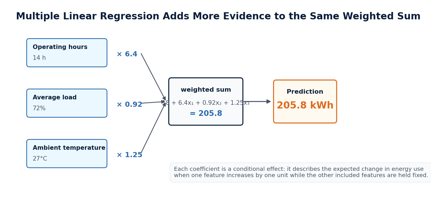 Multiple linear regression combines several weighted features
Suppose the fitted model is:
For a machine-day with:
we obtain:
How to interpret a coefficient
The coefficient means:
Among observations with the same included load percentage and ambient temperature, increasing operating time by one hour is associated with an expected increase of 6.4 kWh.
The phrase “holding the other included variables fixed” is essential.
A coefficient is not automatically causal. If important variables are omitted, measurements are biased, or the data were generated by a selection process, the coefficient may describe association rather than intervention.
8. Multiple Linear Regression Code
import pandas as pd

from sklearn.linear_model import LinearRegression
from sklearn.metrics import mean_absolute_error, r2_score, root_mean_squared_error
from sklearn.model_selection import train_test_split


RANDOM_STATE = 42
FEATURE_COLUMNS = [
    "operating_hours",
    "average_load_pct",
    "ambient_temperature_c",
]
TARGET_COLUMN = "energy_kwh"


data = pd.read_csv("machine_energy.csv")

X = data[FEATURE_COLUMNS]
y = data[TARGET_COLUMN]

X_train, X_test, y_train, y_test = train_test_split(
    X,
    y,
    test_size=0.25,
    random_state=RANDOM_STATE,
)

model = LinearRegression()
model.fit(X_train, y_train)

predictions = model.predict(X_test)

print("MAE:", mean_absolute_error(y_test, predictions))
print("RMSE:", root_mean_squared_error(y_test, predictions))
print("R²:", r2_score(y_test, predictions))

coefficient_table = pd.DataFrame(
    {
        "feature": FEATURE_COLUMNS,
        "coefficient": model.coef_,
    }
)
print(coefficient_table)

new_machine_day = pd.DataFrame(
    [
        {
            "operating_hours": 14.0,
            "average_load_pct": 72.0,
            "ambient_temperature_c": 27.0,
        }
    ]
)

predicted_energy = model.predict(new_machine_day)[0]
print(f"Predicted energy: {predicted_energy:.2f} kWh")
The full runnable example in source_code/example.py creates a reproducible dataset, trains simple and multiple regression models, evaluates them, and adds Lasso and Ridge cross-validation.
9. Main Weaknesses of Ordinary Linear Regression
Ordinary least squares is a strong baseline, but it is not automatically appropriate for every dataset.
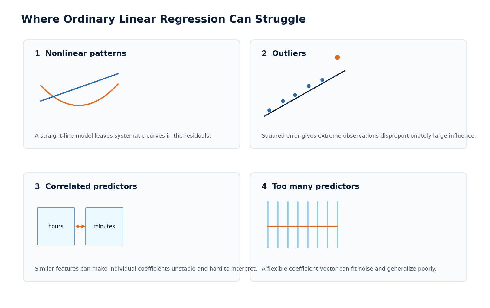 Four common weaknesses of ordinary linear regression
9.1 A linear function may be too simple
The model assumes that the expected target is a linear combination of the supplied features.
If energy use rises slowly at first and then sharply near maximum machine load, a single constant slope will leave a systematic curved pattern in the residuals. The model is then underfitting the relationship, even when its training error appears reasonable.
9.2 Squared loss is sensitive to outliers
Because the loss squares every residual, one extreme observation can contribute more to the objective than many ordinary observations combined.
A faulty meter reading or an unusual shutdown day can pull the fitted line toward itself and distort predictions for typical machine-days.
9.3 Correlated predictors make coefficients unstable
operating_hours and runtime_minutes contain almost the same information. When both are included, many coefficient combinations can produce nearly identical predictions.
Predictions may remain acceptable while individual coefficients change sharply across samples. This makes coefficient interpretation unreliable and is a common symptom of multicollinearity.
9.4 Too many predictors can increase variance
When the number of candidate features is large relative to the amount of training data, ordinary least squares can assign coefficients to accidental noise.
Training error may continue to decrease while test error increases. The fitted model becomes too dependent on the particular sample used for training.
9.5 Extrapolation can be unreliable
A line fitted on machines operating between 4 and 20 hours can still return a number for 30 hours, but that number is outside the region supported by the data.
The physical process may change beyond the observed range, so the model's numerical output should not be mistaken for evidence.
9.6 Predictive association is not causation
A coefficient describes the relationship found after conditioning on the included features. It does not prove that deliberately changing a feature will change the target by that amount.
Omitted variables, selection effects, and measurement bias can create associations that are not causal.
9.7 Statistical conclusions require additional assumptions
The model can always calculate coefficients when the numerical problem is solvable. However, confidence intervals, hypothesis tests, and standard errors require assumptions about sampling, dependence, variance, and model specification.
A useful prediction equation and a valid inferential analysis are related but different goals.
10. How to Address These Weaknesses
The appropriate response depends on the failure mode. Regularization is important, but it solves only a subset of linear regression's weaknesses.
| Weakness | Practical response |
|---|---|
| The relationship is not linear in the supplied features | Add scientifically justified transformations, interactions, polynomial features, or splines; compare with nonlinear models when necessary |
| Squared loss is dominated by outliers | Audit data quality, examine influential observations, transform the target when justified, or use robust losses and robust regression |
| Predictors are strongly correlated | Remove duplicate measurements, combine related features, improve data collection, or use Ridge to stabilize coefficients |
| There are many weak or noisy predictors | Use Lasso for sparse feature selection, Ridge for broad shrinkage, or Elastic Net when both behaviors are useful |
| Predictions require extrapolation | Restrict the deployment range, collect data in the required region, or add valid physical constraints |
| The goal is causal interpretation | Use stronger study design, domain knowledge, experiments, or causal-inference methods rather than relying on regression coefficients alone |
| Error assumptions are violated | Use appropriate diagnostics and, when justified, robust standard errors, clustered methods, generalized least squares, or time-series models |
The next two methods focus specifically on unstable or overly flexible coefficient estimates:
- Lasso adds an absolute-value penalty and can remove some features by setting their coefficients to zero.
- Ridge adds a squared-coefficient penalty and shrinks all coefficients smoothly, which is especially useful for correlated predictors.
Neither method automatically fixes nonlinear structure, corrupted observations, causal bias, unsupported extrapolation, or distribution shift.
11. Lasso Regression: Shrink and Select
Lasso regression adds an penalty:
where:
- is the feature vector for observation
- contains the feature coefficients
- controls penalty strength
- the intercept is usually not penalized
The first term rewards accurate predictions. The second makes large absolute coefficient values expensive.
The absolute-value penalty has a sharp corner at zero. Because of this geometry, the fitted solution can place some coefficients exactly at zero.
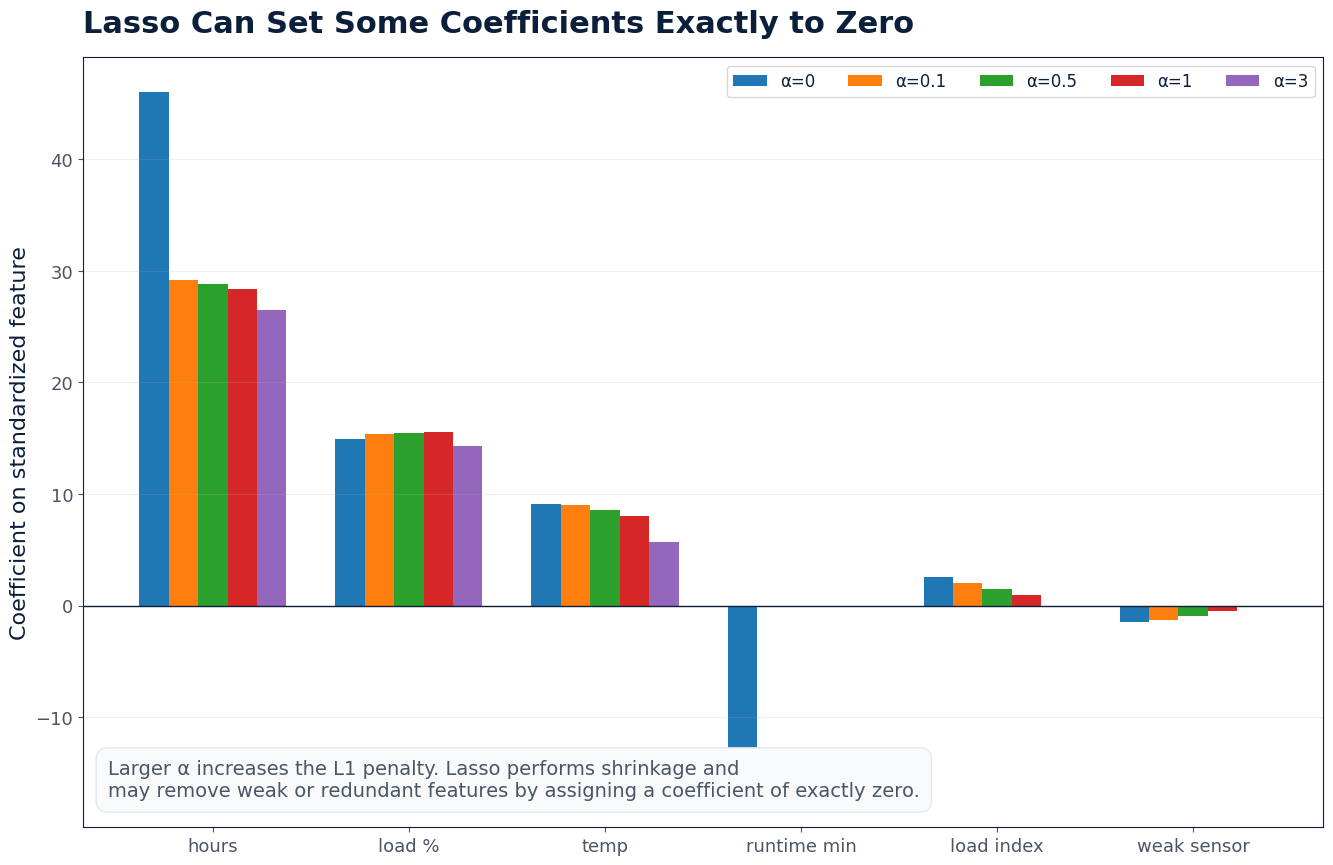 Lasso regression can produce exactly zero coefficients
Why Lasso helps
Lasso is useful when:
- many candidate features may be irrelevant
- a sparse model is valuable for deployment or communication
- automatic feature selection is part of the modeling goal
For the machine-energy example, a weak sensor or a redundant derived variable may receive a coefficient of exactly zero.
What Lasso does not guarantee
When several predictors are strongly correlated, Lasso may select one and suppress another somewhat arbitrarily. The selected feature set can change across training samples.
A zero coefficient means the feature was not selected by this fitted model under this penalty strength. It does not prove that the feature has no physical relationship with energy use.
12. Ridge Regression: Shrink All Coefficients
Ridge regression adds an penalty:
The first term asks the model to fit the observations. The second asks it to keep coefficients small.
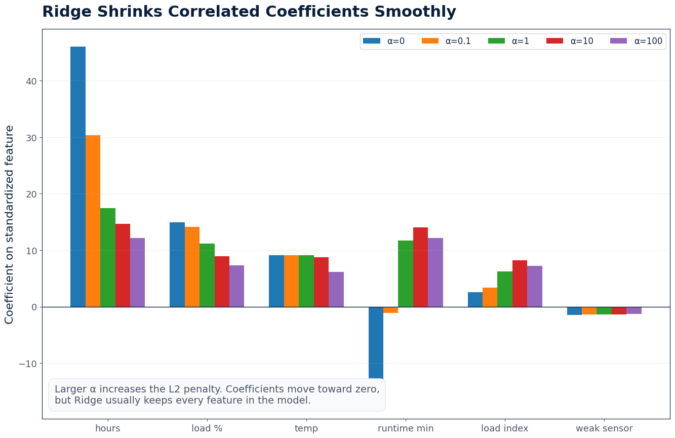 Ridge regression shrinks standardized coefficients
Why Ridge helps
When correlated predictors compete to explain the same signal, ordinary least squares may assign one a large positive coefficient and another a large negative coefficient. Ridge makes such extreme combinations expensive.
This introduces some bias but can substantially reduce variance. The resulting model may make more stable predictions on new observations.
What Ridge does not do
Ridge usually does not remove features. It shrinks coefficients toward zero but typically leaves them nonzero.
Ridge also does not identify which correlated measurement is the uniquely correct explanation. It mainly stabilizes the fitted prediction rule.
13. Lasso vs. Ridge
| Question | Lasso | Ridge |
|---|---|---|
| Penalty | $\alpha\sum_j | \beta_j |
| Main effect | Shrinkage plus possible feature removal | Smooth coefficient shrinkage |
| Exact zero coefficients | Often yes | Usually no |
| Correlated predictors | May select one and suppress others | Tends to distribute weight across them |
| Typical goal | Sparse model and feature selection | Stable prediction and lower coefficient variance |
| Need feature scaling? | Yes | Yes |
Neither method is universally better. The choice should reflect the modeling goal and be evaluated with the same validation procedure.
Elastic Net combines and penalties. It is often useful when sparsity is desirable but the predictors also contain strongly correlated groups.
14. What Is the Hyperparameter?
The central Lasso and Ridge hyperparameter is the penalty strength, usually written as or .
Parameter vs. hyperparameter
A parameter is learned during model fitting:
- intercept
- coefficients
A hyperparameter controls the fitting procedure and must be selected outside the final coefficient optimization:
- Lasso or Ridge penalty strength
Effect of Alpha
- : no regularization; the objective reduces to ordinary least squares
- small : weak shrinkage
- large : strong shrinkage and greater risk of underfitting
For Lasso, software generally expects a strictly positive value rather than using alpha=0 as an ordinary least-squares solver.
Why scaling matters
Suppose operating hours range from 4 to 20 while runtime minutes range from 240 to 1200. A penalty applied directly to raw coefficients would depend heavily on the measurement units.
Standardization transforms each feature using training-set statistics:
where is the training mean and is the training standard deviation.
After standardization, the penalty compares coefficients attached to similarly scaled features.
The scaler must be fitted only with training data. During cross-validation, it must be fitted separately inside each fold. A scikit-learn Pipeline enforces this workflow.
15. Selecting Alpha with Cross-Validation
Choosing from training error would favor little or no regularization. The penalty must instead be judged by performance on observations not used to estimate the coefficients.
K-fold cross-validation works as follows:
- Split the training data into folds.
- Hold out one fold for validation.
- Fit the complete preprocessing-and-model pipeline on the other folds.
- Evaluate the held-out fold.
- Rotate the held-out fold until every fold has been used once.
- Average the validation metric.
- Repeat for every candidate .
- Select the best , refit on all training data, and evaluate the test set once.
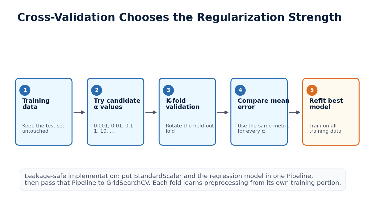 Cross-validation workflow for selecting regularization strength
Leakage-safe Lasso and Ridge code
import numpy as np

from sklearn.linear_model import Lasso, Ridge
from sklearn.model_selection import GridSearchCV
from sklearn.pipeline import Pipeline
from sklearn.preprocessing import StandardScaler


ALPHA_GRID = np.logspace(-3, 3, 49)
CV_FOLDS = 5
RANDOM_STATE = 42


def build_regularized_search(model_name: str) -> GridSearchCV:
    if model_name == "lasso":
        regressor = Lasso(
            max_iter=50_000,
            tol=1e-5,
            random_state=RANDOM_STATE,
        )
    elif model_name == "ridge":
        regressor = Ridge()
    else:
        raise ValueError("model_name must be 'lasso' or 'ridge'.")

    pipeline = Pipeline(
        steps=[
            ("scaler", StandardScaler()),
            ("regressor", regressor),
        ]
    )

    return GridSearchCV(
        estimator=pipeline,
        param_grid={"regressor__alpha": ALPHA_GRID},
        scoring="neg_root_mean_squared_error",
        cv=CV_FOLDS,
        n_jobs=-1,
        refit=True,
    )
Training Lasso:
lasso_search = build_regularized_search("lasso")
lasso_search.fit(X_train, y_train)

best_lasso = lasso_search.best_estimator_
best_lasso_alpha = lasso_search.best_params_["regressor__alpha"]
test_predictions = best_lasso.predict(X_test)
Training Ridge:
ridge_search = build_regularized_search("ridge")
ridge_search.fit(X_train, y_train)

best_ridge = ridge_search.best_estimator_
best_ridge_alpha = ridge_search.best_params_["regressor__alpha"]
test_predictions = best_ridge.predict(X_test)
scikit-learn uses a negative RMSE score because its model-selection interface maximizes scores. The candidate with the value closest to zero has the lowest RMSE.
What should remain untouched?
The test set must not influence:
- feature scaling
- feature selection
- alpha selection
- model comparison
- stopping decisions
Use it once at the end to estimate final generalization performance.
16. Practical Model-Selection Guidance
A disciplined progression is:
- Fit ordinary linear regression as a baseline.
- Inspect residuals and test performance.
- Add scientifically justified features or transformations.
- Use Lasso when a sparse feature set is valuable.
- Use Ridge when coefficient instability or broad shrinkage is the main concern.
- Consider Elastic Net when correlated feature groups and sparsity are both important.
- Select hyperparameters with cross-validation.
- Compare all candidates on the same untouched test set.
- Report uncertainty and operational limitations, not only a single metric.
A regularized model is not automatically better. When the dataset is large, the feature set is small, and multicollinearity is mild, ordinary least squares may perform just as well and remain easier to interpret.
17. Complete Practical Implementation
The accompanying program demonstrates:
- reproducible machine-energy data creation
- a train/test split
- simple linear regression
- multiple linear regression
- Lasso and Ridge pipelines
- standardization inside cross-validation
- alpha selection with
GridSearchCV - MAE, RMSE, and
- coefficient reporting
- one new prediction
Run it from the package directory:
python source_code/example.py
The program intentionally includes redundant and weak predictors. This makes Lasso sparsity and Ridge shrinkage visible in a realistic modeling workflow.
18. Connecting Code to the Main Ideas
| Modeling concept | Python object or method |
|---|---|
| Feature table | pandas DataFrame containing feature columns |
| Target vector | pandas Series containing energy_kwh |
| Fit ordinary linear regression | LinearRegression().fit(X_train, y_train) |
| Numeric prediction | model.predict(X_new) |
| Intercept | model.intercept_ |
| Coefficients | model.coef_ |
| Lasso penalty | Lasso(alpha=...) |
| Ridge penalty | Ridge(alpha=...) |
| Standardization | StandardScaler() |
| Leakage-safe combined workflow | Pipeline(...) |
| Candidate alpha values | param_grid |
| Cross-validation search | GridSearchCV(...) |
| Selected alpha | best_params_["regressor__alpha"] |
| Final refitted pipeline | best_estimator_ |
| Absolute prediction error | mean_absolute_error |
| Root mean squared error | root_mean_squared_error |
| Relative improvement over the mean baseline | r2_score |
All three regressors return numeric predictions. Their outputs are not probabilities, confidence intervals, or causal effects.
19. Key Takeaways
Prediction rules
Simple linear regression:
Multiple linear regression:
Learning objective
Ordinary least squares selects coefficients that minimize squared residuals:
Main weaknesses
Linear regression can underfit nonlinear relationships, react strongly to outliers, produce unstable coefficients with correlated predictors, and overfit when many weak features are available.
Lasso
Lasso shrinks coefficients and can set some exactly to zero, producing a sparse model.
Ridge
Ridge shrinks coefficients smoothly and is especially useful when predictors are correlated or coefficient estimates have high variance.
Hyperparameter selection
The penalty strength controls the trade-off between fitting the training data and shrinking the coefficients. Select it through cross-validation with preprocessing inside a pipeline.
Final warning
A fitted equation is not automatically a trustworthy model. Validation, residual inspection, data quality, deployment range, and the distinction between prediction and causation still matter.