Hard-Margin Support Vector Machines: Choosing the Widest Safe Linear Boundary

Learning Objectives

By the end of this lesson, you should be able to:

1. Explain why finding any separating boundary is not enough when several valid boundaries exist.
2. Distinguish a raw linear score, a Logistic Regression probability, a functional margin, and a geometric distance.
3. Derive the distance from a point to a linear decision boundary.
4. Explain why the SVM margin must be normalized by $\lVert w\rVert$.
5. Build the hard-margin SVM objective from the maximum-margin idea.
6. Interpret the constraints $y_i(w^Tx_i+b)\geq1$ geometrically.
7. Explain why support vectors, rather than all training observations equally, determine the final boundary.
8. Describe what hard-margin SVM guarantees, when it has no solution, and what it does not provide.
9. Train and inspect a linear SVM with a leakage-safe scikit-learn workflow.

Scope of this lesson

This lesson studies hard-margin SVM only. We assume that the training data is linearly separable. Slack variables, the penalty parameter $C$, hinge-loss optimization, and soft-margin SVM are intentionally reserved for the next lesson.

1. The Remaining Problem: Which Correct Boundary Should We Choose?

Consider an automated quality-control system that classifies manufactured parts from two measurements:

• $x_1$: a surface-defect score
• $x_2$: a dimension-deviation score

Each part is represented by a feature vector:

The label is:

A small teaching dataset is:

The two classes can be separated by a straight line. That sounds like a problem the Perceptron has already solved.

The Perceptron searches for parameters $w$ and $b$ that make every training example land on the correct side of:

If the data is linearly separable, the Perceptron eventually finds a separating boundary. Its convergence theorem does not say that the boundary is unique, centered between the classes, or stable under small changes in the inputs.

Logistic Regression addressed a different weakness. It kept the same linear score,

but transformed that score into an estimated probability through the sigmoid function. This made the output more interpretable for ranking risk and selecting decision thresholds.

However, Logistic Regression optimizes log loss. It does not explicitly ask:

Among all lines that separate the training examples, which line leaves the largest geometric safety gap?

That is the question hard-margin Support Vector Machines answer.

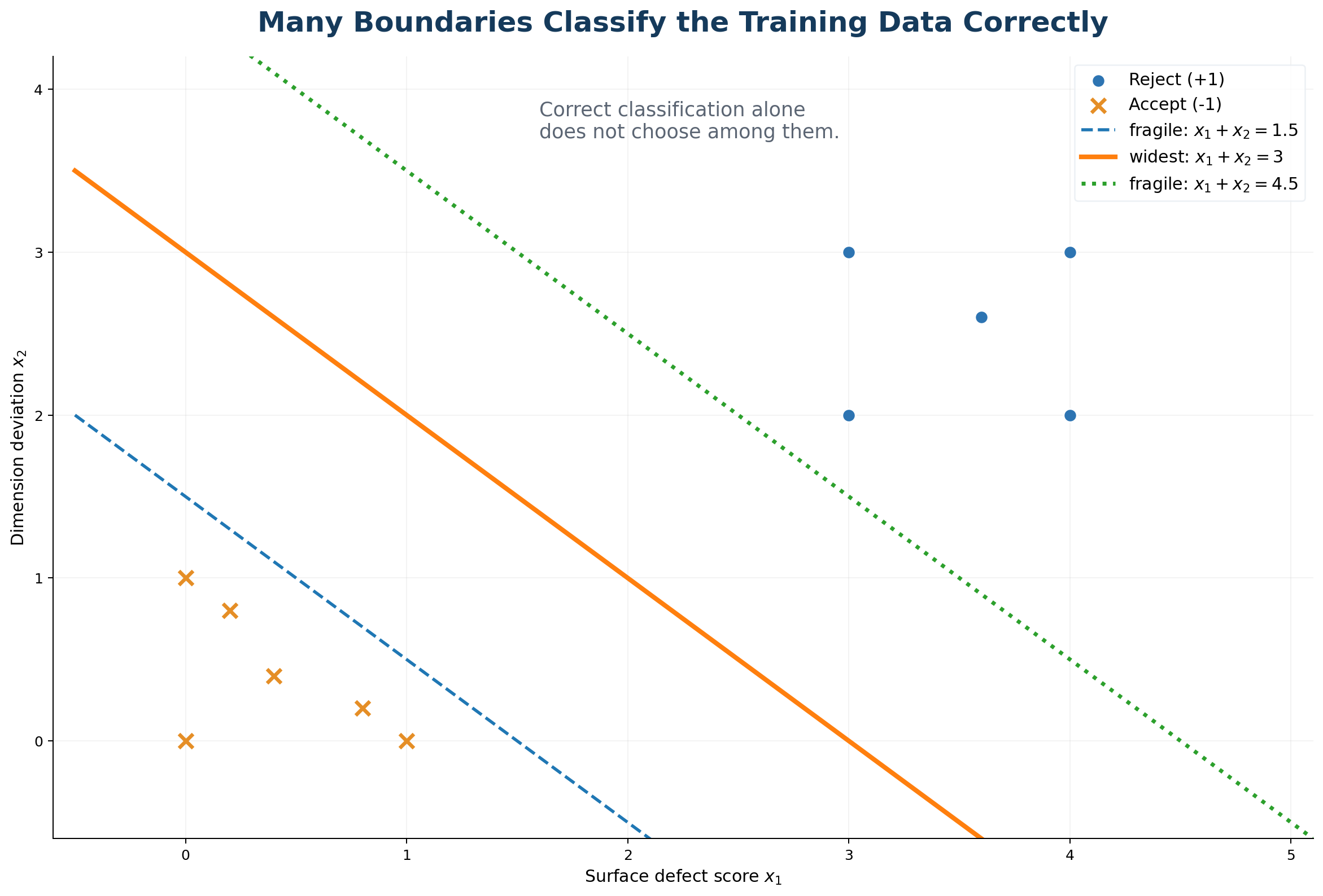
Diagram teaching notes

What appears: The same separable dataset with three different linear boundaries.
What to notice: Every line classifies the displayed training observations correctly, but the two outer lines pass very close to one class.
What to explain: Correctness is a feasibility condition, not yet a rule for choosing the best feasible boundary.
Connection: The next step is to replace “find any separator” with a measurable preference for one separator.

Concept Check

A model classifies every training example correctly. Does that prove the boundary is the most robust separating boundary?

No. It only proves that the boundary is feasible. Another feasible boundary may leave a larger gap between the classes.

2. What Carries Over from the Perceptron and Logistic Regression?

Hard-margin SVM is not a completely different kind of predictor. It begins with the same linear decision function:

where:

• $x\in\mathbb{R}^d$ is the feature vector,
• $w\in\mathbb{R}^d$ is the weight vector,
• $b\in\mathbb{R}$ is the bias or intercept,
• $f(x)\in\mathbb{R}$ is the raw decision score.

The predicted class is:

Thus:

produces class $+1$, while:

produces class $-1$.

The decision boundary is the set of inputs for which:

In two dimensions, this is a line. In three dimensions, it is a plane. In higher dimensions, it is a hyperplane.

2.1 What do $w$ and $b$ do geometrically?

The vector $w$ is perpendicular to the decision boundary. It is therefore called a normal vector to the hyperplane.

• Changing the direction of $w$ rotates the boundary.
• Changing $b$ shifts the boundary.
• Multiplying both $w$ and $b$ by the same positive constant does not change the boundary.

That last point will become essential.

Suppose:

The boundary is:

Now multiply both parameters by $5$:

The new equation is:

Dividing by $5$ gives the original line. The geometry has not changed.

2.2 What is different from Logistic Regression?

Logistic Regression interprets:

as an estimated probability under a probabilistic model.

Hard-margin SVM does not apply the sigmoid and does not fit a probability model. It uses the geometry of the score relative to the separating boundary.

A probability and a geometric distance answer different questions:

• Probability: Under the fitted probabilistic model, how much probability is assigned to a class?
• Geometric distance: How far is this input from the hyperplane in the chosen feature space?
• Raw score: What value does the unnormalized linear function produce?

Common mistake — “Logistic Regression already chooses the best boundary.”

Logistic Regression chooses parameters that reduce log loss. Hard-margin SVM chooses parameters that maximize the smallest geometric distance from the training data to the boundary. The objectives are different, so their fitted boundaries need not be the same.

Common mistake — “A probability of 0.9 means the point is 0.9 units from the boundary.”

Probability and geometric distance use different scales and different mathematical meanings. Neither can be substituted for the other.

3. Why Correct Separation Alone Is Not Enough

For the quality-control data, consider boundaries of the form:

The acceptable parts satisfy:

for the closest displayed acceptable observations, while the closest reject observation satisfies:

Therefore, any value:

creates a valid separating boundary.

Three possibilities are:

All three classify the training examples correctly.

The first line passes only a short distance from the acceptable class. The third line passes only a short distance from the reject class. The middle line is centered between the closest observations from the two classes.

3.1 Fragility near a boundary

Suppose an acceptable part lies close to a boundary. A small amount of sensor noise could move its measured position across the line, changing the prediction even though the underlying part has not meaningfully changed.

A boundary with more empty space around it can tolerate a larger perturbation before the prediction flips.

This motivates a stronger objective:

Do not merely separate the training examples. Choose the separating hyperplane whose nearest training observation is as far away as possible.

This empty region is the margin.

3.2 What a wider margin does and does not mean

A wider training margin provides a geometric form of robustness. If a training point is a distance $\gamma$ from the boundary, any perturbation shorter than $\gamma$ cannot cross the boundary when measured in the same feature-space geometry.

This does not guarantee that:

• every future observation will be classified correctly,
• the model is probabilistically confident,
• the chosen features represent the real problem well,
• the deployment distribution matches the training distribution.

The margin gives a principled boundary-selection rule. It is not a universal guarantee of good predictions.

Concept Check

Why not choose the boundary that is farthest from the positive class only?

Because doing so could place the boundary extremely close to the negative class. The relevant quantity is the distance to the closest observation from either class.

4. From a Linear Score to Distance from the Hyperplane

To maximize separation, we need to measure distance. The raw score:

is not yet a geometric distance because its magnitude changes when $w$ and $b$ are rescaled.

4.1 Why the raw score cannot be the distance

Take the boundary:

and the point:

Using:

the score is:

Using the equivalent parameters:

the score is:

The physical point and the geometric boundary are unchanged, so the distance cannot have changed from $3$ units to $15$ units. We need a normalization that removes this arbitrary scaling.

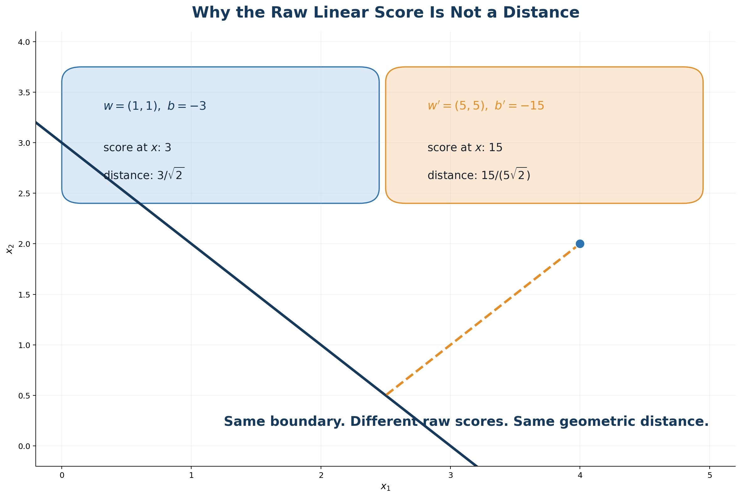
Diagram teaching notes

What appears: One point and one boundary described by two different parameter pairs.
What to notice: The raw score changes by a factor of five, but the normalized distance does not change.
What to explain: A valid geometric quantity must be invariant to equivalent parameter scaling.
Connection: This motivates dividing the score by $\lVert w\rVert$.

4.2 Deriving the distance formula

Let the hyperplane be:

For a point $x$, the shortest path to the hyperplane must be perpendicular to the hyperplane. Because $w$ is normal to the hyperplane, the closest point $x^\star$ must lie somewhere along the direction of $w$.

Write:

where $t$ tells us how far to move in the normal direction.

Because $x^\star$ lies on the boundary:

Substitute $x^\star=x-tw$:

Distribute $w^T$:

Since:

we have:

Solving for $t$:

The displacement from $x$ to $x^\star$ is:

Its length is:

Substitute the expression for $t$:

Therefore:

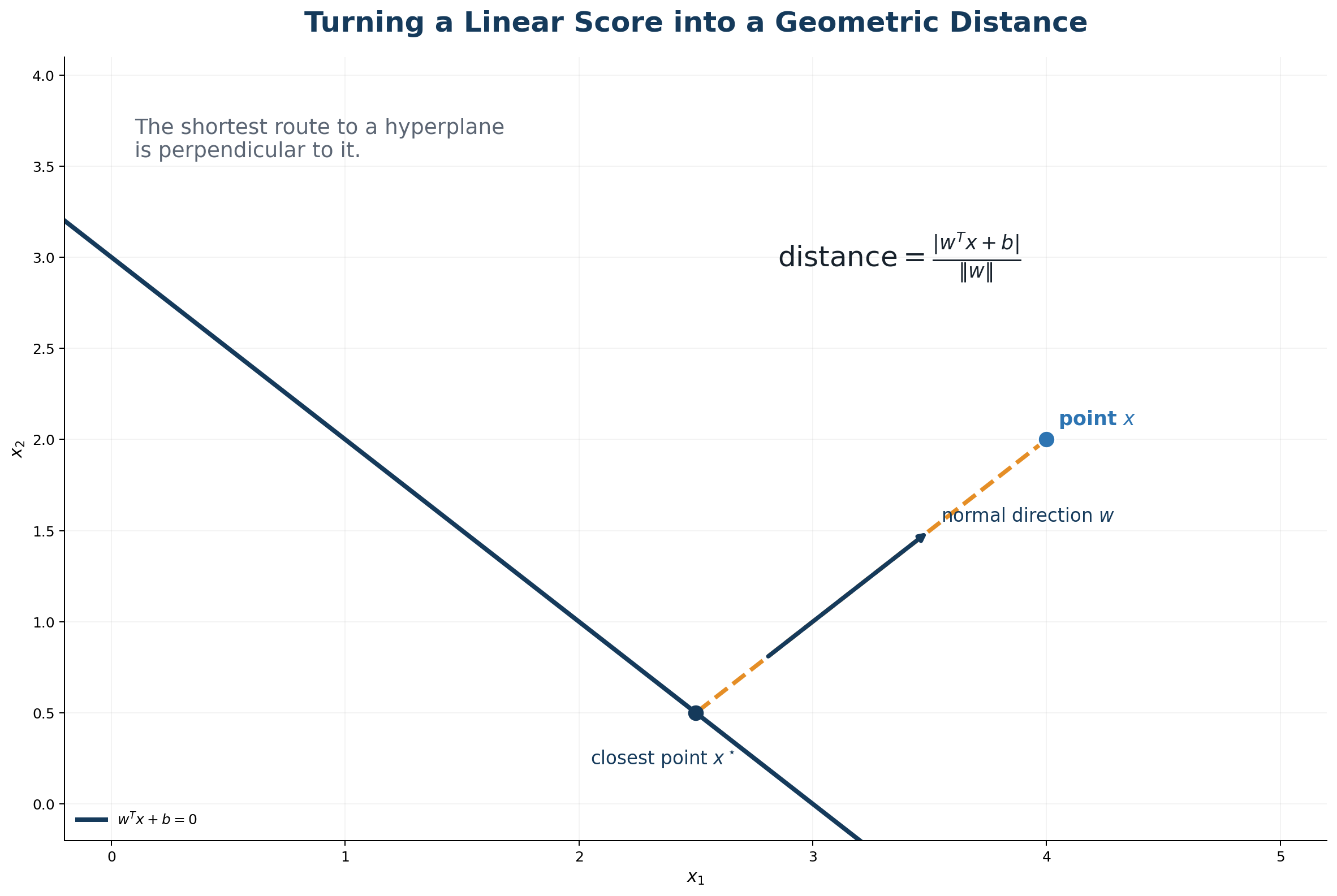
Diagram teaching notes

What appears: A point, its perpendicular projection onto the boundary, and the normal direction $w$.
What to notice: The shortest segment is parallel to $w$, not parallel to either coordinate axis.
What to explain: The numerator gives a signed algebraic score; the denominator converts it into geometric units.
Connection: The next section adds the class label so that “correct side” and “incorrect side” are handled in one expression.

4.3 Numerical distance calculation

For:

the score is $3$, and:

Therefore:

Using $w'=5w$ and $b'=5b$:

The distance is unchanged, as required.

Common mistake — “A larger raw score always means a larger geometric distance.”

For one fixed fitted model, score magnitude and distance are proportional because $\lVert w\rVert$ is fixed. Across different parameter scalings or different models, raw scores cannot be compared as distances unless they are normalized by $\lVert w\rVert$.

5. Functional Margin and Geometric Margin

The distance formula uses an absolute value, but classification also requires the side of the boundary.

For a labeled example $(x_i,y_i)$, define the functional margin:

where $y_i\in\{-1,+1\}$.

5.1 Why multiply by the label?

If $y_i=+1$, correct classification requires:

Multiplying by $+1$ keeps the value positive.

If $y_i=-1$, correct classification requires:

Multiplying by $-1$ makes the result positive.

Therefore:

means the example is on the correct side, while:

means it is on the wrong side.

The functional margin combines both label cases into one expression.

5.2 Why the functional margin is still not geometric

If $w$ and $b$ are multiplied by $5$, the functional margin is also multiplied by $5$, even though the boundary does not move.

The geometric margin of example $i$ is therefore:

This is a signed distance measured toward the example's correct class side.

• $\gamma_i>0$: correctly classified
• $\gamma_i=0$: exactly on the decision boundary
• $\gamma_i<0$: misclassified

For a separating boundary, every training example has a positive geometric margin.

5.3 Margin of the complete training dataset

A boundary is only as safe as its closest training example. The margin of the dataset with respect to $(w,b)$ is:

where:

• $n$ is the number of training examples,
• $i$ indexes one training example,
• the minimum selects the closest correctly classified observation.

Hard-margin SVM seeks the boundary that maximizes this minimum distance.

Common mistake — “The average distance should be maximized.”

A large average could hide one observation that is almost touching the boundary. The minimum distance directly controls the narrowest part of the safety gap.

Common mistake — “SVM distance is a probability-like confidence score.”

The geometric margin is measured in the geometry of the feature space. It is not constrained to $[0,1]$, does not sum across classes, and is not automatically calibrated as a probability.

6. From Maximum Margin to the Hard-Margin SVM Objective

We can now write the boundary-selection goal directly:

subject to every example being correctly classified.

This expression captures the right idea, but it is inconvenient to optimize because:

• it contains a minimum over observations,
• it contains a ratio,
• the same boundary has infinitely many equivalent parameter scalings.

The next step uses the scaling freedom deliberately.

6.1 Canonical scaling

For any separating hyperplane, all functional margins are positive. Because multiplying $(w,b)$ by a positive constant leaves the boundary unchanged, we may choose a scale at which the smallest functional margin is exactly $1$:

This convention is called canonical scaling.

Under this scale, every training example satisfies:

At least one observation satisfies equality.

Now the dataset's geometric margin becomes:

Because the minimum numerator is $1$:

Therefore maximizing the margin is equivalent to minimizing $\lVert w\rVert$.

6.2 Why minimize the squared norm?

Instead of minimizing:

we minimize:

This produces the same optimal $w$ because squaring is monotone for nonnegative values. The square is smoother and easier to differentiate. The factor $1/2$ cancels the $2$ that appears when differentiating the squared norm:

The factor does not change the location of the optimum.

6.3 The hard-margin primal problem

The complete optimization problem is:

Every component has a distinct role.

Objective

Minimizing the norm makes:

as large as possible. This widens the distance from the decision boundary to the closest training observations.

Constraints

The constraints require every training example to:

1. be classified correctly, and
2. lie on or beyond its class's margin boundary.

For $y_i=+1$:

For $y_i=-1$:

The two margin hyperplanes are therefore:

and:

The decision boundary lies halfway between them:

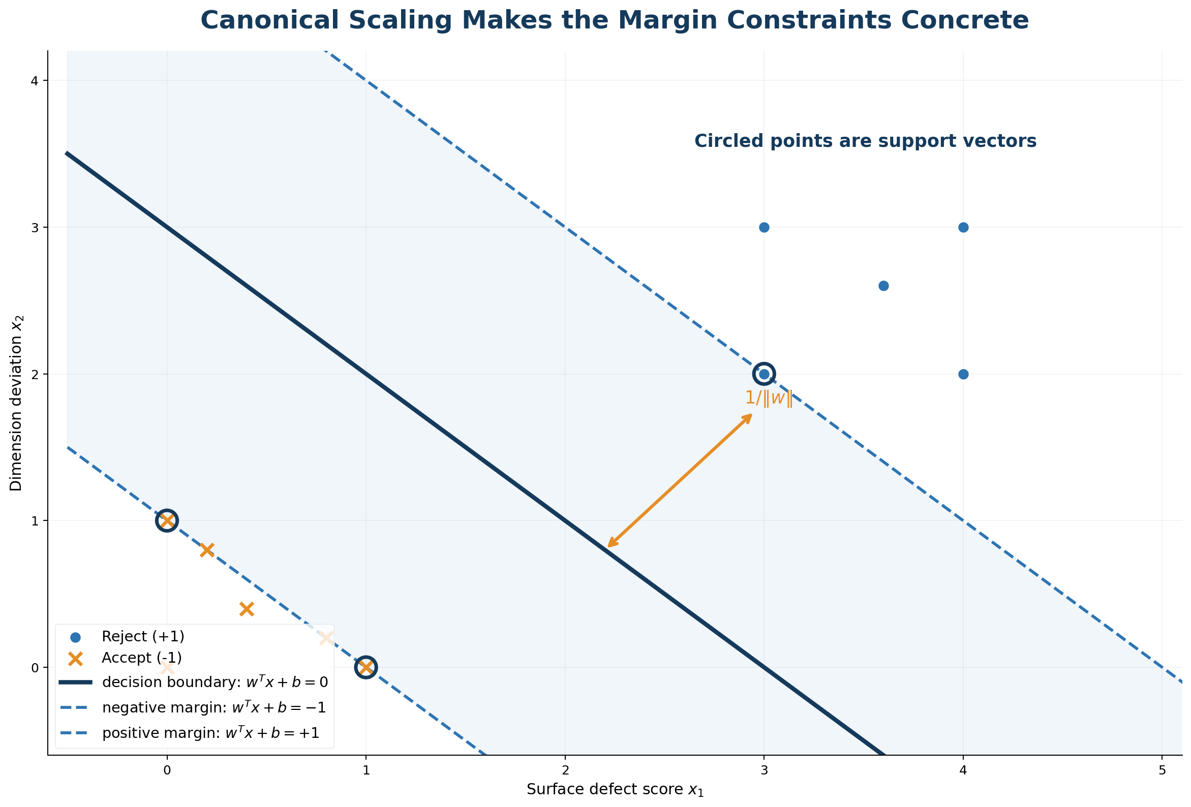
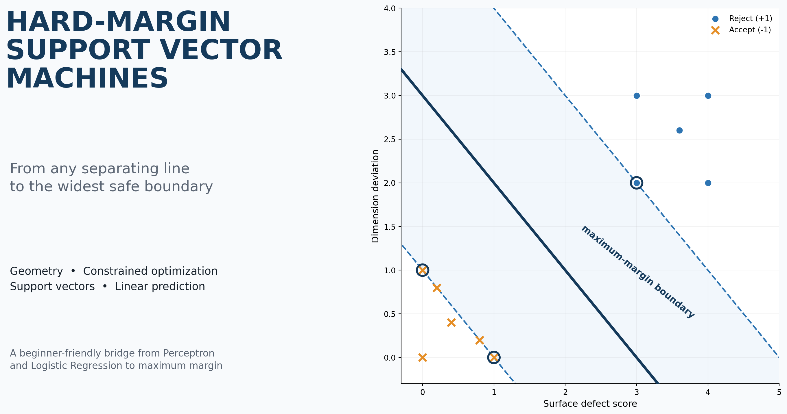
Diagram teaching notes

What appears: The decision boundary, the two canonical margin hyperplanes, the margin band, and circled closest observations.
What to notice: No training point lies inside the band. The closest points touch its edges.
What to explain: The constraints define feasibility; the norm objective widens the band while preserving feasibility.
Connection: The touching observations will be named support vectors because they support the optimal band.

6.4 Margin to one side versus full margin width

The distance from the decision boundary:

to either margin hyperplane is:

The distance from the negative margin hyperplane to the positive margin hyperplane is:

Both quantities are called “the margin” in different explanations.

This lesson uses:

• margin to the nearest training point: $\frac{1}{\lVert w\rVert}$
• full margin width: $\frac{2}{\lVert w\rVert}$

Always check which convention is being used.

6.5 Why the constraints are essential

Suppose we minimized only:

without classification constraints. The smallest possible norm would be obtained by:

That does not define a useful separating boundary.

The objective alone prefers a small weight vector. The constraints force the small-norm solution to remain a valid separator.

Checkpoint Interpretation

Hard-margin SVM is not “minimize the weights” by itself. It is:

Find the smallest-norm weight vector among all parameter choices that keep every training observation on the correct side of the margin.

7. Manual Walkthrough: Solving a Two-Feature Example

Return to the quality-control dataset.

The closest acceptable observations lie on:

The closest reject observation is:

which lies on:

The line centered between these two parallel lines is:

Written as a decision function:

This boundary is geometrically correct, but it is not yet in canonical scale. We need the closest positive example to have score $+1$ and the closest negative examples to have score $-1$.

Choose:

Then:

The decision boundary is still:

Multiplying by $2$ gives $x_1+x_2-3=0$, so the same line is represented.

7.1 Verify the closest acceptable observations

For:

the score is:

The functional margin is:

The constraint is active exactly at equality.

For:

the same calculation gives a functional margin of $1$.

7.2 Verify the closest reject observation

For:

the score is:

The functional margin is:

This constraint is also active.

7.3 Verify noncritical observations

For the reject observation:

the score is:

Its functional margin is $2>1$. It lies beyond the positive margin hyperplane and is not one of the closest observations.

The constraint table is:

7.4 Compute the margin

The norm of $w$ is:

The distance from the boundary to the nearest training observation is:

The full margin width is:

The optimization objective at this solution is:

7.5 Compare with off-center boundaries

For a line:

the distance from a point with coordinate sum $s$ is:

For $c=2$:

• nearest acceptable distance: $\frac{|1-2|}{\sqrt{2}}\approx0.707$
• nearest reject distance: $\frac{|5-2|}{\sqrt{2}}\approx2.121$
• dataset margin: $0.707$

For $c=3$:

• nearest acceptable distance: $\frac{|1-3|}{\sqrt{2}}\approx1.414$
• nearest reject distance: $\frac{|5-3|}{\sqrt{2}}\approx1.414$
• dataset margin: $1.414$

For $c=4$:

• nearest acceptable distance: $\frac{|1-4|}{\sqrt{2}}\approx2.121$
• nearest reject distance: $\frac{|5-4|}{\sqrt{2}}\approx0.707$
• dataset margin: $0.707$

The centered boundary maximizes the minimum distance.

7.6 Complete prediction for a new part

Consider:

The raw score is:

Because the score is positive:

The part is predicted to be rejected.

Its signed geometric distance is:

This is a distance in the chosen feature space, not a probability.

Common mistake — “Every future observation must be outside the margin.”

The hard-margin constraints apply to the training observations used to fit the model. A new observation can fall inside the margin band and still receive a class prediction based on the sign of its score.

8. How the Hard-Margin SVM Learns

The Perceptron learns through local mistake-driven updates. Hard-margin SVM is defined differently: it solves a constrained optimization problem over the complete training dataset.

8.1 The optimization is a quadratic program

The objective:

is quadratic in $w$.

Each constraint:

is linear in the parameters $w$ and $b$.

An optimization problem with a quadratic objective and linear constraints is a quadratic program.

8.2 Why constrained optimization is necessary

There are two simultaneous goals:

1. Keep every training observation on the correct side of its margin boundary.
2. Make the weight norm as small as possible so the geometric margin becomes large.

Neither goal can replace the other.

• Constraints without an objective leave many feasible boundaries.
• The norm objective without constraints gives the useless solution $w=0$.
• Together, they define one principled selection problem.

8.3 Convexity and the global solution

The squared norm is a convex function. The feasible region defined by linear inequalities is also convex.

This matters because a convex optimization problem has no inferior local minima. If a numerical solver converges to an optimum that satisfies the constraints, it has reached a global optimum of the stated hard-margin problem.

The optimal weight vector $w$ is unique because the objective is strictly convex in $w$. In unusual degenerate configurations, more than one bias value may describe the same optimal orientation while satisfying the constraints, although typical datasets pin down $b$ through support vectors from both classes.

Convexity does not guarantee strong performance on unseen data. It guarantees that the mathematical training problem is solved globally.

8.4 What a solver does conceptually

A practical quadratic-programming or SVM solver conceptually performs the following work:

1. Starts with candidate parameters or dual coefficients.
2. Checks how the constraints and objective behave.
3. Adjusts the candidate solution.
4. Moves toward a feasible point with smaller $\lVert w\rVert^2$.
5. Stops when optimization conditions are satisfied within a numerical tolerance.

Libraries often use specialized decomposition or coordinate-optimization methods rather than a simple full-batch gradient descent loop. Therefore, “one epoch” is not the defining unit of hard-margin SVM learning.

8.5 Language-independent algorithm

Input:
    linearly separable training examples (x_i, y_i)
    labels y_i in {-1, +1}

1. Place features on meaningful, comparable scales.

2. Define the optimization problem:
       minimize (1/2) * ||w||^2
       subject to y_i * (w^T x_i + b) >= 1
       for every training example i

3. Solve the constrained convex quadratic program.

4. Identify training examples satisfying:
       y_i * (w^T x_i + b) = 1
   These are the support vectors.

5. For a new input x:
       score = w^T x + b
       predict +1 if score > 0
       predict -1 if score < 0

6. When a geometric distance is needed:
       distance = score / ||w||

Optimization Checkpoint

Hard-margin SVM does not repeatedly repair only the latest mistake. It selects parameters by optimizing a global geometric objective under constraints from every training example.

9. Support Vectors: The Observations That Hold the Boundary in Place

At the optimum, some observations satisfy:

These points lie exactly on one of the margin hyperplanes. They are called support vectors.

The name is geometric: these observations support the widest feasible margin band. If the band expanded any farther without rotating or shifting appropriately, it would run into one of them.

Observations satisfying:

lie beyond the margin. They are correctly classified with extra geometric room.

9.1 Why non-support observations often do not move the boundary

Imagine moving a training observation that lies far beyond the margin. If it remains correctly classified and does not become one of the closest points, the current optimum still satisfies its constraint. The observation does not tighten the feasible region near the optimum, so the boundary may remain unchanged.

9.2 Why moving a support vector can change the boundary

A support vector is part of the closest geometry between the two classes. Moving it can:

• change the nearest distance,
• change the orientation that produces the widest gap,
• change the bias,
• cause another observation to become a support vector.

The boundary does not have to change after every support-vector movement in every symmetric or redundant configuration, but support vectors are the observations with direct potential to determine the optimum.

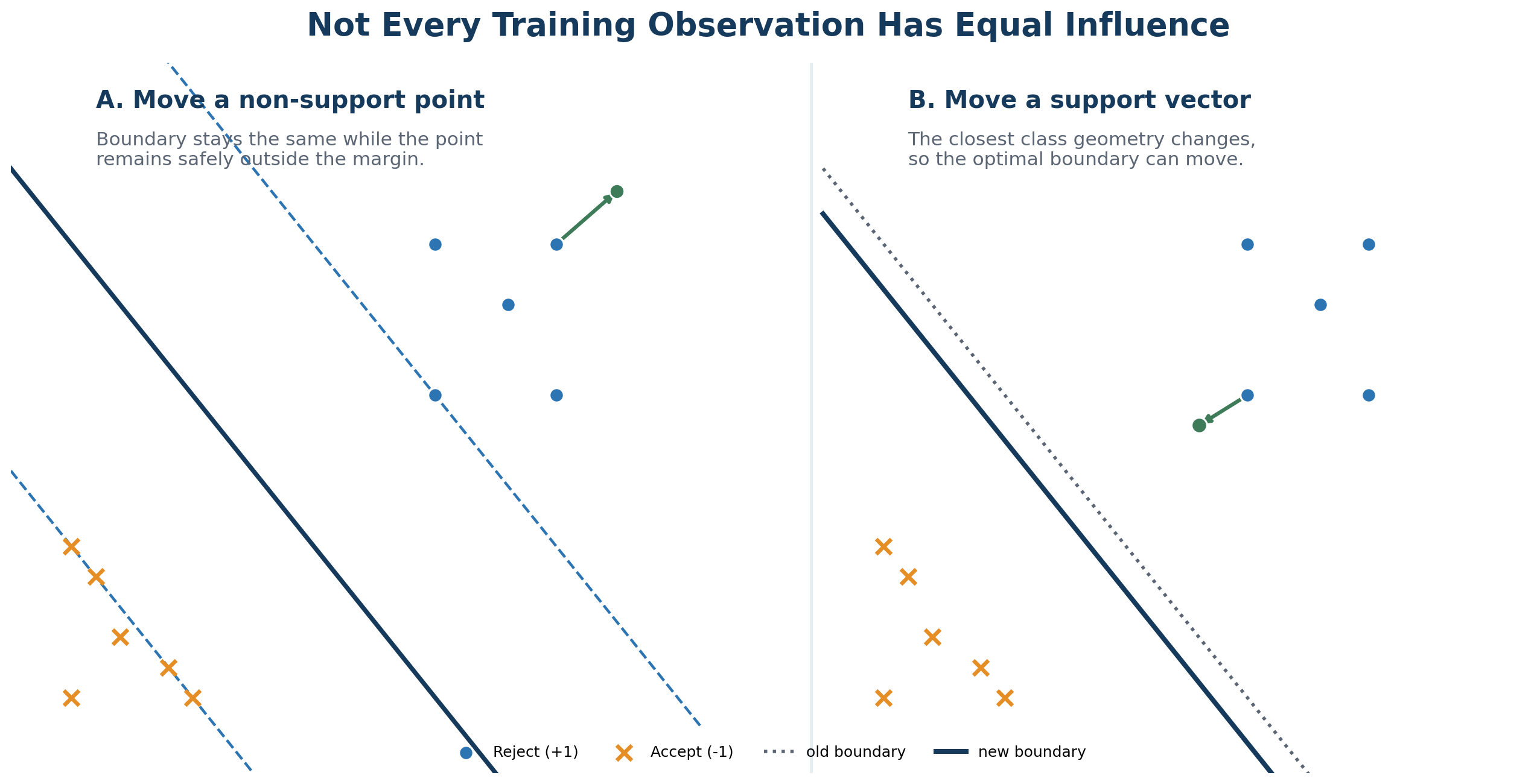
Diagram teaching notes

What appears: One scene moves a non-support observation; another moves a support vector.
What to notice: The first movement leaves the closest class geometry unchanged, while the second changes it.
What to explain: Constraints that are loose at the optimum exert no immediate pressure; active constraints define the edge of feasibility.
Connection: Lagrange multipliers provide the mathematical version of this “pressure” interpretation.

Common mistake — “All training observations contribute equally.”

All observations create constraints, but only active constraints directly hold the optimal margin in place. Non-support observations can matter if they move far enough to become active.

Common mistake — “The boundary changes whenever any training point moves.”

A small movement of a non-support observation may leave the solution exactly unchanged. The important question is whether the closest class geometry or active constraints change.

10. Why Support Vectors Appear: An Accessible Dual View

The primal formulation already defines hard-margin SVM:

A deeper question remains:

Can we show mathematically that the final weight vector is built from the observations that press against the margin?

Lagrange multipliers answer this question.

10.1 Rewriting the constraints

Write each constraint as:

Associate a nonnegative multiplier $\alpha_i\geq0$ with it.

Intuitively, $\alpha_i$ measures how strongly the $i$-th constraint participates in holding the optimum in place.

The Lagrangian is:

The first term is the margin objective. The second term incorporates the constraints.

10.2 Stationarity with respect to $w$

At the optimum, differentiate with respect to $w$ and set the result to zero:

Therefore:

This equation says that the final normal vector is a weighted combination of training observations.

10.3 Stationarity with respect to $b$

Differentiate with respect to $b$:

Therefore:

The weighted influence of the positive and negative classes must balance in this sense.

10.4 Complementary slackness

A key optimality condition is:

This product can be zero in two main ways.

Case 1: The observation lies outside the margin

If:

then:

For the product to be zero:

That observation disappears from the weighted expression for $w$.

Case 2: The multiplier is positive

If:

then complementary slackness requires:

so:

The observation lies on a margin hyperplane and is a support vector.

This is the mathematical reason only a subset of observations directly determines $w$.

10.5 The dual optimization problem

Substituting the stationarity conditions into the Lagrangian gives the dual form:

Every symbol has already appeared:

• $\alpha_i$ is the multiplier for observation $i$,
• $y_i$ is its label,
• $x_i^Tx_j$ is the dot product between two observations.

The dual is not required to make predictions with a linear hard-margin SVM. Its main teaching value here is that it exposes two important facts:

1. The model depends directly on support vectors with nonzero coefficients.
2. The observations appear through dot products.

The second fact will become important when nonlinear SVMs are introduced later. No nonlinear transformation is needed for the current hard-margin linear lesson.

Concept Check

If a training observation satisfies $y_i(w^Tx_i+b)=2.4$, what does complementary slackness imply about its multiplier?

Because the constraint is strictly satisfied, $\alpha_i=0$. It is not an active support vector.

11. When Does Hard-Margin SVM Work?

Hard-margin SVM requires a feasible separator satisfying:

for every training observation after an appropriate positive rescaling of the parameters.

This is possible exactly when the training data is linearly separable in the chosen feature representation.

11.1 Conditions that support a meaningful solution

Hard-margin SVM is most appropriate when:

• a linear hyperplane can perfectly separate the training labels,
• labels are reliable,
• extreme observations are credible rather than data errors,
• the feature representation captures the relevant structure,
• feature units create a meaningful geometry,
• training observations reasonably represent deployment cases.

11.2 What the optimization guarantees

When the constraints are feasible, the hard-margin problem finds a global maximum-margin linear separator.

More precisely, it finds a feasible hyperplane that maximizes:

This gives a principled answer to the non-uniqueness problem left by the Perceptron.

11.3 What it does not guarantee

The maximum training margin does not guarantee:

• the lowest possible test error,
• calibrated class probabilities,
• robustness to distribution shift,
• correct labels,
• fairness across subgroups,
• a nonlinear boundary,
• immunity to unusual support observations.

The guarantee is about the stated optimization problem, not every property desired from a deployed classifier.

11.4 One conflicting observation can make the problem infeasible

Real datasets may contain overlap, measurement noise, or incorrect labels. A single negative-labeled observation placed inside the positive region can make perfect linear separation impossible.

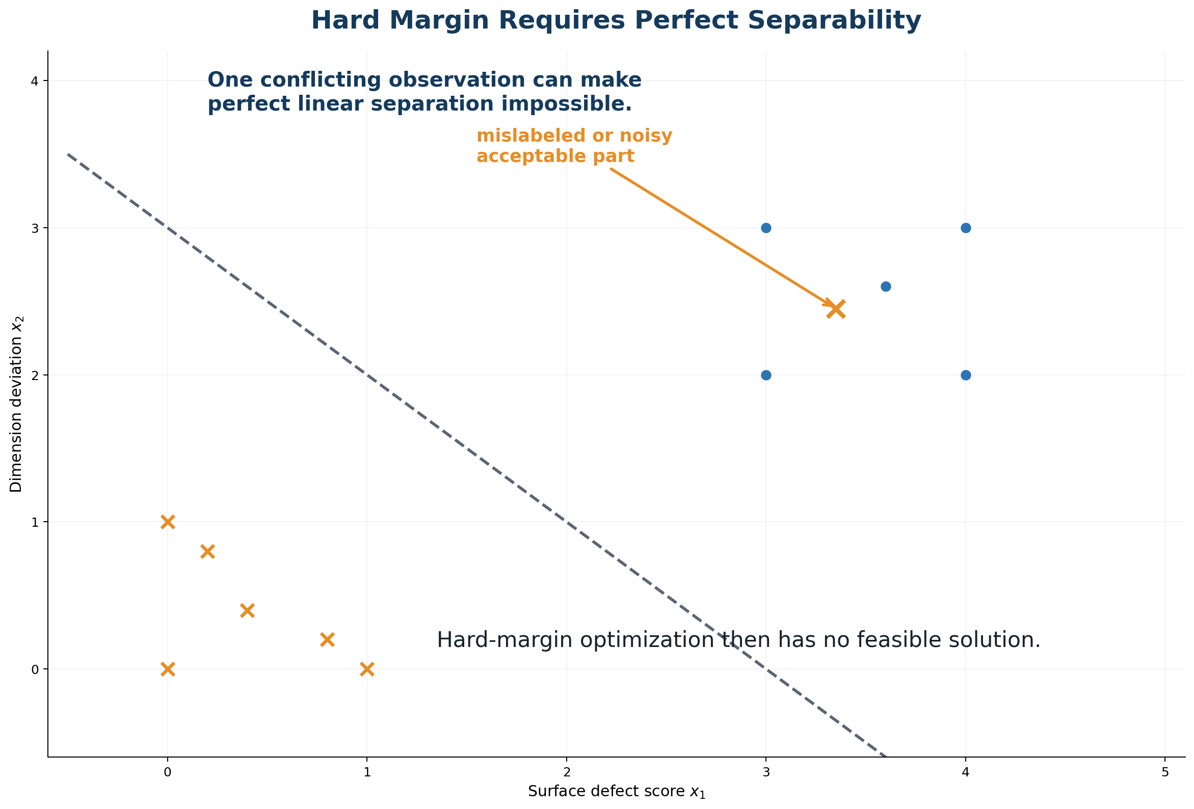
Diagram teaching notes

What appears: A previously separable dataset with one conflicting acceptable label inside the reject cluster.
What to notice: No straight line can place all positive examples on one side and all negative examples on the other.
What to explain: Hard-margin SVM does not trade margin against mistakes; it declares this set of constraints infeasible.
Connection: The next SVM extension will relax the perfect-separation requirement, but that extension is outside the current lesson.

Common mistake — “A wider margin always means zero training errors.”

In hard-margin SVM, zero training errors are required before the margin is optimized. A wide margin does not cause the zero-error condition; the constraints enforce it.

Common mistake — “Increase $C$ to make hard-margin SVM better.”

The mathematical hard-margin formulation has no penalty parameter $C$. $C$ belongs to soft-margin formulations. A library may use a very large $C$ to numerically approximate hard-margin behavior on separable data, but increasing it indefinitely is not a general performance guarantee.

12. Limitations and the Next Improvements

The maximum-margin principle solves an important Perceptron limitation, but hard-margin SVM still has boundaries.

12.1 It cannot learn a nonlinear boundary in the original feature space

The prediction rule remains:

A single linear hyperplane cannot represent patterns such as concentric classes or XOR without changing the feature representation.

12.2 It has no feasible solution for nonseparable training data

Overlap, label noise, and contradictory observations can make the constraints impossible to satisfy.

This is the most immediate practical limitation of hard margin.

12.3 The solution can be controlled by a small number of extreme observations

Support-vector sparsity is useful, but it also means that unusual closest observations can strongly determine the margin and orientation.

The maximum-margin boundary is optimal for the observed feature-space geometry. If a support vector is a measurement error or unrepresentative outlier, the learned boundary may be undesirable for deployment.

12.4 It does not produce probabilities

The outputs of:

model.decision_function(X)

are signed scores. After normalization by $\lVert w\rVert$, they are signed geometric distances in the model's feature space.

Neither output is automatically a class probability.

12.5 It is sensitive to feature scale

The SVM objective uses Euclidean length:

and geometric distance in feature space. Changing a feature from meters to millimeters changes the numerical geometry unless preprocessing compensates for it.

A model can run without standardization, but then its margin reflects the arbitrary measurement units. Scaling is therefore usually essential unless the units are intentionally chosen to encode relative importance.

12.6 Short preview of later improvements

The next lesson should begin with the second row: how to preserve the maximum-margin idea when perfect separation is unrealistic.

13. Perceptron, Logistic Regression, and Hard-Margin SVM

All three methods can use the same linear score:

Their central difference is not the prediction formula. It is what they optimize and how they interpret the output.

13.1 Probabilistic confidence versus geometric confidence

Suppose two models place an observation on the positive side.

Logistic Regression may report:

Hard-margin SVM may report a signed geometric distance of:

These values are not competing estimates of the same quantity.

• The Logistic Regression value is a model-based probability estimate.
• The SVM value says the point is $1.7$ scaled feature-space units from the boundary.
• The reliability of the probability must be checked through calibration.
• The usefulness of the distance depends on the feature representation and scaling.

13.2 Does Logistic Regression ever produce the same boundary?

It can, but it is not guaranteed. The two methods solve different objectives.

On some symmetric datasets, their decision boundaries may look nearly identical. On other datasets, especially when observations are distributed unevenly away from the class frontier, the boundaries can differ because Logistic Regression continues to account for all observations through log loss while hard-margin SVM is determined by its support vectors.

14. Practical Implementation with scikit-learn

scikit-learn's SVC implements $C$-Support Vector Classification. It does not expose a separate “infinite-$C$” hard-margin estimator.

For a clean, linearly separable teaching dataset, a very large value of C can approximate the hard-margin solution. This is an implementation device, not a new theoretical component of the hard-margin formulation.

The workflow below:

1. creates named feature columns,
2. splits before preprocessing,
3. standardizes inside a Pipeline,
4. trains a linear SVM,
5. evaluates predictions,
6. inspects support vectors,
7. computes normalized geometric distances,
8. predicts one new part.

from __future__ import annotations

import numpy as np
import pandas as pd
from sklearn.metrics import accuracy_score
from sklearn.model_selection import train_test_split
from sklearn.pipeline import Pipeline
from sklearn.preprocessing import StandardScaler
from sklearn.svm import SVC

RANDOM_STATE = 42
TEST_SIZE = 0.25
HARD_MARGIN_APPROXIMATION_C = 1_000_000.0

FEATURE_COLUMNS = [
    "surface_defect_score",
    "dimension_deviation",
]

ACCEPT_LABEL = -1
REJECT_LABEL = 1


def create_dataset() -> tuple[pd.DataFrame, pd.Series]:
    """Create a small, linearly separable quality-control dataset."""
    rows = [
        # Acceptable parts (-1)
        (0.0, 0.0, ACCEPT_LABEL),
        (1.0, 0.0, ACCEPT_LABEL),
        (0.0, 1.0, ACCEPT_LABEL),
        (0.4, 0.4, ACCEPT_LABEL),
        (0.8, 0.2, ACCEPT_LABEL),
        (0.2, 0.8, ACCEPT_LABEL),
        (1.1, 0.3, ACCEPT_LABEL),
        (0.3, 1.1, ACCEPT_LABEL),
        (0.8, 0.8, ACCEPT_LABEL),
        (1.2, 0.5, ACCEPT_LABEL),
        (0.5, 1.2, ACCEPT_LABEL),
        (1.0, 1.0, ACCEPT_LABEL),
        # Reject parts (+1)
        (3.0, 2.2, REJECT_LABEL),
        (3.2, 2.4, REJECT_LABEL),
        (3.5, 2.0, REJECT_LABEL),
        (3.0, 3.0, REJECT_LABEL),
        (4.0, 2.2, REJECT_LABEL),
        (3.8, 3.0, REJECT_LABEL),
        (4.2, 2.8, REJECT_LABEL),
        (3.6, 3.6, REJECT_LABEL),
        (4.5, 3.2, REJECT_LABEL),
        (3.2, 3.8, REJECT_LABEL),
        (4.0, 4.0, REJECT_LABEL),
        (4.6, 3.8, REJECT_LABEL),
    ]

    frame = pd.DataFrame(
        rows,
        columns=[*FEATURE_COLUMNS, "quality_label"],
    )
    X = frame[FEATURE_COLUMNS].copy()
    y = frame["quality_label"].copy()
    return X, y


def build_model() -> Pipeline:
    """Build a leakage-safe scaling and linear-SVM pipeline."""
    return Pipeline(
        steps=[
            ("scaler", StandardScaler()),
            (
                "classifier",
                SVC(
                    kernel="linear",
                    C=HARD_MARGIN_APPROXIMATION_C,
                    probability=False,
                ),
            ),
        ]
    )


def signed_geometric_distance(
    model: Pipeline,
    X: pd.DataFrame,
) -> np.ndarray:
    """Return signed distance to the learned boundary in scaled space."""
    scaler: StandardScaler = model.named_steps["scaler"]
    classifier: SVC = model.named_steps["classifier"]

    X_scaled = scaler.transform(X)
    raw_scores = classifier.decision_function(X_scaled)
    weight_norm = np.linalg.norm(classifier.coef_.ravel())

    if weight_norm == 0:
        raise ValueError("The learned weight vector has zero norm.")

    return raw_scores / weight_norm


def main() -> None:
    X, y = create_dataset()

    X_train, X_test, y_train, y_test = train_test_split(
        X,
        y,
        test_size=TEST_SIZE,
        random_state=RANDOM_STATE,
        stratify=y,
    )

    model = build_model()
    model.fit(X_train, y_train)

    train_predictions = model.predict(X_train)
    test_predictions = model.predict(X_test)

    print(
        "Training accuracy:",
        f"{accuracy_score(y_train, train_predictions):.3f}",
    )
    print(
        "Test accuracy:",
        f"{accuracy_score(y_test, test_predictions):.3f}",
    )

    classifier: SVC = model.named_steps["classifier"]
    weight_norm = np.linalg.norm(classifier.coef_.ravel())
    margin_to_boundary = 1.0 / weight_norm
    full_margin_width = 2.0 / weight_norm

    print("Number of support vectors:", classifier.n_support_.sum())
    print("Margin to nearest support hyperplane:", f"{margin_to_boundary:.3f}")
    print("Full margin width:", f"{full_margin_width:.3f}")

    support_positions = classifier.support_
    support_rows = X_train.iloc[support_positions].copy()
    support_rows["label"] = y_train.iloc[support_positions].to_numpy()

    print("\nSupport-vector training rows:")
    print(support_rows.to_string(index=False))

    new_part = pd.DataFrame(
        [
            {
                "surface_defect_score": 3.4,
                "dimension_deviation": 2.5,
            }
        ]
    )

    raw_score = float(model.decision_function(new_part)[0])
    distance = float(signed_geometric_distance(model, new_part)[0])
    prediction = int(model.predict(new_part)[0])

    print("\nNew part:")
    print(f"Raw decision score: {raw_score:.3f}")
    print(f"Signed geometric distance: {distance:.3f}")
    print(
        "Prediction:",
        "Reject" if prediction == REJECT_LABEL else "Accept",
    )


if __name__ == "__main__":
    main()

14.1 Why scaling is inside the pipeline

The correct order is:

1. split the original data,
2. fit the scaler using only the training partition,
3. transform the training partition,
4. fit the SVM,
5. apply the same fitted scaler to test and future observations.

Placing StandardScaler inside Pipeline makes this workflow automatic. Test-set statistics are not used to fit the scaler.

14.2 Why the distance is computed after scaling

The classifier is trained in standardized feature space. Its coef_ and decision_function() therefore describe that space.

The normalized quantity:

is a geometric distance in standardized units.

It is not the same as a distance measured directly in the original raw measurement units.

14.3 Inspecting support vectors

For SVC, the attribute:

classifier.support_

contains the positions of the training observations selected as support vectors.

The attribute:

classifier.n_support_

reports how many support vectors belong to each class.

For a linear kernel:

classifier.coef_

contains the learned weight vector.

14.4 Why probability=False

Hard-margin SVM does not intrinsically produce probabilities.

Enabling probability estimation in SVC adds a separate calibration procedure. That output should not be presented as part of the hard-margin derivation.

14.5 Interpreting the example output

One run of the included script produced:

Training accuracy: 1.000
Test accuracy: 1.000
Number of support vectors: 2
Margin to nearest support hyperplane: 0.781
Full margin width: 1.562

Support-vector training rows:
 surface_defect_score  dimension_deviation  label
                  1.0                  1.0     -1
                  3.0                  2.2      1

New part:
Raw decision score: 1.436
Signed geometric distance: 1.121
Prediction: Reject

The perfect accuracy on this small synthetic split is expected because the data was deliberately constructed to be easy and separable. It is not evidence of real-world model quality.

15. Connecting the Code to the Mathematics

Implementation warning

A very large C is safe only as a teaching approximation on clean, separable data. On noisy or nonseparable data, it can create numerical and modeling problems. That behavior belongs to the soft-margin discussion.

16. Key Takeaways

The prediction rule is still linear

Hard-margin SVM uses the same kind of decision boundary as the Perceptron and binary Logistic Regression.

The remaining problem was boundary selection

The Perceptron can find any separator. Logistic Regression optimizes probability-based log loss. Neither objective explicitly selects the widest geometric gap among all feasible separators.

Raw score is not geometric distance

Normalization by $\lVert w\rVert$ removes arbitrary parameter scaling.

The geometric margin uses the label

The label makes positive geometric margin mean “on the correct side” for both classes.

Canonical scaling produces the hard-margin constraints

The nearest observations satisfy equality.

The hard-margin objective is

Minimizing the norm maximizes the margin while the constraints preserve perfect separation.

Support vectors determine the boundary

Support vectors satisfy:

They are the active observations that hold the maximum-margin solution in place.

The method has a strict success condition

Hard-margin SVM requires linearly separable training data. If overlap, noise, or contradictory labels make the constraints infeasible, the method has no solution.

Geometric confidence is not probability

The decision score and normalized distance do not represent $P(y=1\mid x)$.

The next problem is realistic imperfection

Real data is rarely perfectly separable. The natural next question is:

How can we preserve the maximum-margin principle while allowing limited margin violations or classification errors?

That question leads to soft-margin SVM.

Glossary

Active constraint
A constraint that holds with equality at the optimum. For hard-margin SVM, support-vector constraints are active.

Bias $b$
The intercept that shifts the decision boundary without directly changing its normal direction.

Canonical scaling
A parameter scaling in which the smallest training functional margin equals $1$.

Constraint
A requirement that every feasible solution must satisfy. Hard-margin SVM requires $y_i(w^Tx_i+b)\geq1$.

Convex optimization
Optimization in which the objective and feasible region have geometry that prevents inferior local minima.

Decision boundary
The set of points satisfying $w^Tx+b=0$.

Dual problem
An alternative optimization formulation expressed through Lagrange multipliers $\alpha_i$.

Functional margin
The scale-dependent quantity $y_i(w^Tx_i+b)$.

Geometric margin
The normalized signed distance $y_i(w^Tx_i+b)/\lVert w\rVert$.

Hard-margin SVM
A maximum-margin linear classifier that requires every training example to be perfectly separated.

Hyperplane
A linear decision boundary in an arbitrary number of dimensions.

Lagrange multiplier $\alpha_i$
A nonnegative coefficient associated with a constraint. Nonzero coefficients identify observations that directly influence the SVM solution.

Margin hyperplanes
Under canonical scaling, the parallel hyperplanes $w^Tx+b=+1$ and $w^Tx+b=-1$.

Normal vector $w$
A vector perpendicular to the decision boundary.

Quadratic program
An optimization problem with a quadratic objective and linear constraints.

Support vector
A training observation that lies on a margin hyperplane and helps determine the optimal boundary.

Weight vector $w$
The learned coefficients that determine the orientation and feature contributions of the linear decision function.